Pick the node $n$ with the smallest $f(n)$ from the frontier, where $f$ is an estimate of the total cost to the optimal solution passing through that node.
Best-first search selects nodes from the frontier with the smallest $f(n)$ where $f(n)$ estimates the total cost to the optimal solution passing through that node. What’s a useful way to “split up” $f$?
$h$ the future cost, when it is an estimate this is $A^\ast$ search and $h$ is the heuristic
Best-first search selects nodes from the frontier with the smallest $f(n)$ where $f(n)$ estimates the total cost to the optimal solution passing through that node. How are BFS and UCS special cases of this?
Using the heuristic function $h$ encodes domain knowledge about the problem.
Can you give an @example where a more accurate heuristic (in terms of being closer in absolute value to the perfect heuristic) actually causes $A^\ast$ to fail to be optimal?
Clearly the optimal solution is $\mathbf{InitialState} \to \mathbf R \to \mathbf{GoalState}$. Here are two heuristic functions, $h _ >$ and $h _ {\ll}$, which could be used with $A^\ast$:
$h _ >$ leads to the solution $\mathbf{InitialState} \to \mathbf L \to \mathbf{GoalState}$ whereas $h _ \ll$ leads to $\mathbf{InitialState} \to \mathbf R \to \mathbf{GoalState}$. The problem is that the highlighted entry makes $h _ >$ not admissible.
@State an important theorem about $A^\ast$ search and admissible heuristics.
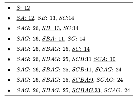
Suppose you want to solve a $A^\star$ tree search problem manually. What’s a convenient way of writing down the frontier and the order nodes are expanded?
function A*GraphSearch(problem, frontier) returns (solution or failure):
	explored = {}
	Insert(RootNode(problem.InitialState), frontier)
	while the frontier is not empty:
		node = Remove(frontier) # Here node removed with least f value
		add node.State to explored
		if problem.GoalTest(node.State):
			return node
		for each action in problem.Actions(node.State):
			if child.State is not in explored: (*)
				Insert(ChildNode(problem, node, action), frontier)
	return failure
Consider the following code:
function A*GraphSearch(problem, frontier) returns (solution or failure):
	explored = {}
	Insert(RootNode(problem.InitialState), frontier)
	while the frontier is not empty:
		node = Remove(frontier) # Here node removed with least f value
		add node.State to explored
		if problem.GoalTest(node.State):
			return node
		for each action in problem.Actions(node.State):
			if problem.GoalTest(child.State):
				return child

			if child.State is not in explored: (*)
				Insert(ChildNode(problem, node, action), frontier)
	return failure
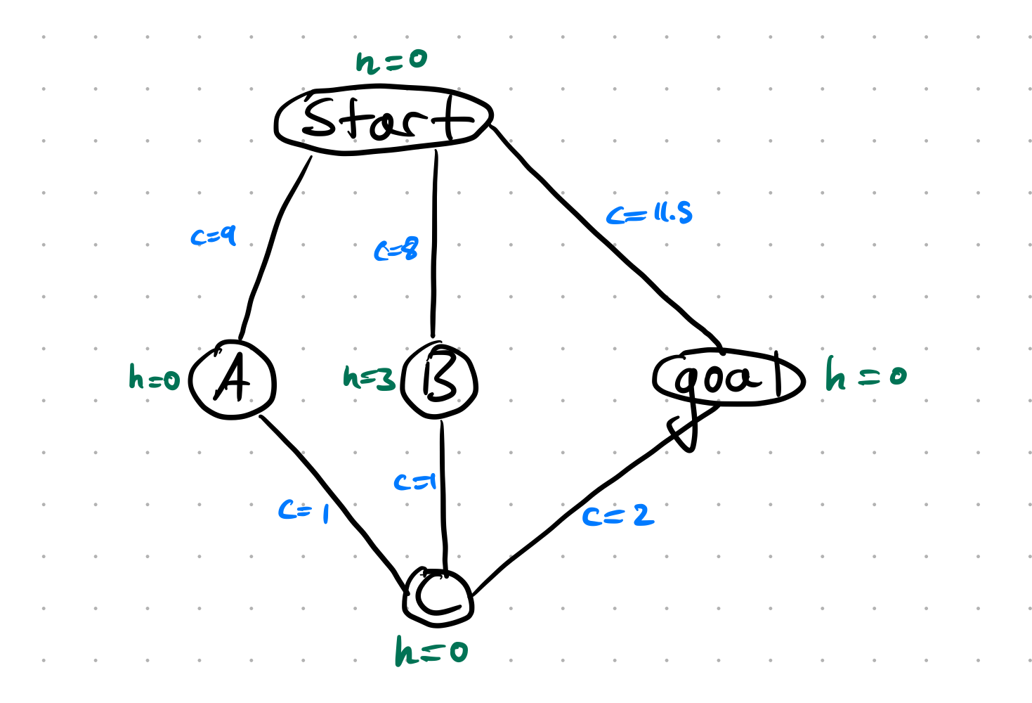
Can you give an @example to show that adding a goal test before adding a node might break optimality?
What’s a useful mental model to have when thinking about $A^\ast$ search, and how could you apply this to e.g. understanding why $A^\ast$ tree search is complete as long as there are only finitely many nodes with $f$-cost less than a goal node?
The threshold starts at the estimate of the cost of the initial state, and increases for each iteration of the algorithm. At each iteration, the threshold used for the next iteration is the minimum cost of all values that exceeded the current threshold.
# h is an admissible heuristic

function IDA*(problem) returns (goal or failure):
	root = RootNode(problem.InitialState)
	f_limit = h(root) # Estimate of cost to solution

	while True:
		# Search for the goal node using the current f_limit
		# If no goal is found, f_limit is updated to the minimum cost
		# of all values found that exceed the previous f_limit.
		goal, f_limit = IDA-DFS(problem, root, f_limit)

		if goal != failure:
			return goal

		if f_limit = infinity:
			return failure

function IDA-DFS(problem, node, f_limit) returns (goal, or next cost):
	# Calculate score for node (total cost so far + estimate cost to goal)
	f_node = g(node) + h(node)

	# If this node exceeds the limit, return failure and also the score
	if f_node > f_limit:
		return (failure, f_node)

	# If this node is a goal, return this node
	if problem.GoalTest(node.State):
		return (node, f_limit)

	# We set the next_f_limit to the minimum cost across all nodes exceeding
	# the current f_limit
	next_f_limit = infinity

	for each action in problem.Actions(node.State):
		succ = ChildNode(problem, node, action)

		# Start a new search from this successor node
		# If there's a failure, new_f_limit will be the minimum across all
		# nodes exceeding the current f_limit
		goal, new_f_limit = IDA-DFS(problem, succ, f_limit)

		if goal != failure:
			return (goal, new_f_limit)

		next_f_limit = min(next_f_limit, new_f_limit)

	return (failure, next_f_limit)
Advantages:
It avoids the overhead of keeping a sorted queue of nodes.
Deriving heuristics
What does it mean for heuristic $h _ 1$ to dominate heuristic $h _ 2$?
Take the admissible heuristic to be the exact solution cost of a relaxed version of the problem, where the optimal solution cost of the relaxed problem is less than or equal to the optimal solution cost of the real problem.
How can you derive an admissible heuristic from subproblems?
Storing the exact solution to disjoint subproblems of a subproblem, and then calculating an admissible heuristic by summing together the optimal solution cost for each subproblem in a given problem.
How can you reduce the amount of nodes that $A^\star$ expands as part of the search tree?
Consider the point at which node $n$ is added to the priority queue.
Then delete from the queue every node $m$ where $g(m) + h(m) > g(n) + u(n)$. Such $m$ cannot lead to a better solution than $n$: The true cost from $n$ is $g(n) + h^\ast(n)$, and hence $g(n) + h^\ast(n) \le g(n) + u(n)$ because $u$ is an upper bound.
The condition ensures that $g(n) + u(n) < g(m) + h(m)$, which implies that $g(n) + h^\ast(n) < g(m) + h(m)$. But then $h$ is admissible since $g(m) + h(m) \le g(m) + h^\ast(m)$, which is the true cost for $m$.
Thus $g(n) + h^\ast(n) < g(m) + h^\ast(m)$ and hence we can safely discard $m$.