Machine Learning MT23, Recurrent neural networks
Outstanding Questions
- The parameters are shared for every unrolled version of an RNN network. Why does running gradient descent on each of these cause updates that work well in general?
Flashcards
What is “sequential data” $\pmb x$, and what neural network architecture is often used to model it?
Where there is a dependence between each input $x _ i$ and each input that came before it $\pmb x _ {<i}$, and recurrent architectures are often used for this.
Suppose we have a language model that assigns a probability to a sequence of words $\pmb w = (w _ 1, \cdots, w _ N)$. What typical “factorisation” of $p(\pmb w)$ is used to simplify the task?
The main task of a language model is to describe a probability distribution $p(\pmb w)$ over sequences of words (called utterances) given by $\pmb w = (w _ 1, \cdots, w _ N)$. Say these words come from an alphabet $\Sigma$. What condition do we have on such a distribution?
What is the intuitive interpretation of the cross entropy of an utterance $w^N _ 1 = (\pmb w _ 1, \cdots, \pmb w _ N)$, given by
\(H(w^N _ 1) = -\frac 1 N \sum^N _ {i =1} \log _ 2(\pmb w _ i)\)
and what is the perplexity given this definition (here each $\pmb w _ i$ is a one-hot encoding of a word)?
The number of bits required to encode each symbol, and perplexity is given by \(\text{perplexity}(w^N _ 1) = 2^{H(w^N _ 1)}\)
A typical “factorisation” of $p(\pmb w)$ used to simplify the task of language models is
\(p(w _ 1, \cdots, w _ N) = p(w _ 1)p(w _ 2 \mid w _ 1)p(w _ 3 \mid w _ 1, w _ 2) \cdots p(w _ N \mid w _ 1, w _ 2, \cdots, w _ N)\)
What happens if we make the Markov assumption for a “unigram” model, and for a “bigram” model?
Unigram: \(p(w _ 1, \cdots, w _ N) \approx p(w _ 1)p(w _ 2)p(w _ 3) \cdots p(w _ N)\) Bigram: \(p(w _ 1, \cdots, w _ N) \approx p(w _ 1)p(w _ 2 \mid w _ 1)p(w _ 3 \mid w _ 2) \cdots p(w _ N \mid w _ {N-1})\)
Suppose we are making a bigram language model so that the probability $p(\pmb w)$ of an utterance is approximated as
\(p(w _ 1, \cdots, w _ N) \approx p(w _ 1)p(w _ 2 \mid w _ 1)p(w _ 3 \mid w _ 1, w _ 2) \cdots p(w _ N \mid w _ {N-2}, w _ {N-1})\)
What would the simplest approach, using a MLE multivariate distribution, model
\(p(w _ 3 \mid w _ 1, w _ 2)\)
as, and what is a disadvantage of this approach?
\(\frac{\text{count}(w _ 1, w _ 2, w _ 3)}{\text{count}(w _ 1, w _ 2)}\) Most utterances end up being assigned zero probability with such a model.
Draw a picture representing a neural trigram network with one hidden layer and then state the forward equations assuming we use softmax as the final activation.
- 4 nodes
- Two inputs, $\pmb w _ 1$ and $\pmb w _ 2$
- One output, $\hat{\pmb p} _ 3$, probability distribution over words in the vocabulary
- One hidden layer $\pmb h$ in the middle
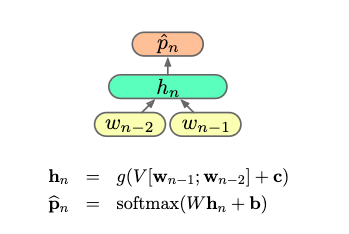
Then forward equations are something like
\[\pmb h = \text{activation}(V[\pmb w _ 1 ; \pmb w _ 2] + \pmb c)\] \[\hat{\pmb p} _ n = \text{softmax}(W\pmb h + \pmb b)\]Suppose we have training data $\pmb w = (\pmb w _ 1, \cdots, \pmb w _ N)$, i.e. a long utterance where each $\pmb w _ i$ is a one-hot encoding of a word. What does the usual training objective look like for a simple language model?
The cross entropy loss of the data given the model, \(-\frac{1}{N} \sum^N _ {i=1} \pmb w _ i^\intercal \log (\hat{\pmb p} _ i)\) (here $\hat{\pmb p} _ i$ does not just depend on $\pmb w _ i$, but on its position in the utterance).
Suppose we have the following trigram network:

Suppose we have training data $\pmb w = (\pmb w _ 1, \cdots, \pmb w _ N)$ i.e. a long utterance where each $\pmb w _ i$ is a one-hot encoding of a word. The standard training objective is the cross-entropy of the data given the model, equal to
\[\mathcal F = -\frac{1}{N} \sum^N _ {i=1} \text{cost}(\pmb w _ i, \hat{\pmb p} _ i)\]
where
\[\text{cost}(\pmb a, \pmb b) = \pmb a^\top \log(\pmb b)\]
Quickly derive an expression for the gradients
\[\frac{\partial \mathcal F}{\partial W}, \frac{\partial \mathcal F}{\partial V}\]
\(\begin{aligned} \frac{\partial \mathcal F}{\partial W} &= \frac{\partial}{\partial W} \left( - \frac 1 N \sum^N _ {i=1} \text{cost} _ i(\pmb w _ i, \hat{\pmb p} _ i) \right) \\\\ &= -\frac 1 N \sum^N _ {i = 1} \frac{\partial \text{cost} _ i(\pmb w _ i, \hat{\pmb p _ i})}{\partial W} \\\\ &= -\frac 1 N \sum^N _ {i = 1} \frac{\partial \text{cost} _ i}{\partial \hat{\pmb p} _ i} \frac{\partial \hat{\pmb p} _ i}{\partial W} \end{aligned}\) (since we’re considering the training data $\pmb w _ i$ fixed), and \(\begin{aligned} \frac{\partial \mathcal F}{\partial V} &= \frac{\partial}{\partial V} \left( - \frac 1 N \sum^N _ {i=1} \text{cost} _ i(\pmb w _ i, \hat{\pmb p} _ i) \right) \\\\ &= -\frac 1 N \sum^N _ {i = 1} \frac{\partial \text{cost} _ i(\pmb w _ i, \hat{\pmb p _ i})}{\partial V} \\\\ &= -\frac 1 N \sum^N _ {i = 1} \frac{\partial \text{cost} _ i}{\partial \hat{\pmb p} _ i} \frac{\partial \hat{\pmb p} _ i}{\partial V} \\\\ &= -\frac 1 N \sum^N _ {i = 1} \frac{\partial \text{cost} _ i}{\partial \hat{\pmb p} _ i} \frac{\partial \hat{\pmb p} _ i}{\partial \pmb h _ i} \frac{\partial \pmb{h} _ i}{\partial V} \end{aligned}\)
Suppose we are using the following recurrent neural network for language modelling:
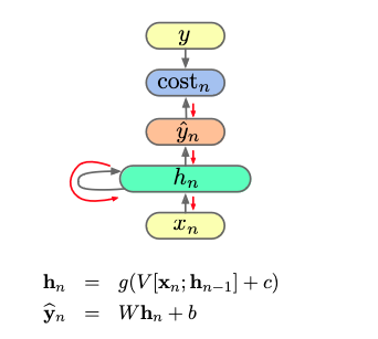
and have training data $\pmb w = (\pmb w _ 1, \cdots, \pmb w _ N)$. This gives us the unrolled computational graph
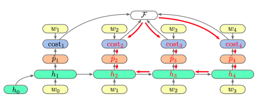
(in the above image, $N = 4$).
The BPTT applies backpropogration to this graph to in order to update the model parameters $V, W, b, c$. Quickly derive a heuristic for when the gradient information linking the effect of $w _ 0$ on $\text{cost} _ N$ will propogate, i.e. when
\(\frac{\partial \text{cost} _ N}{\partial h _ 1}\)
does not explode and does not vanish.
We have
\[\begin{aligned} \frac{\partial \text{cost} _ N}{\partial h _ 1} = \frac{\partial \text{cost} _ N}{\partial \hat{\pmb p} _ N} \frac{\partial \pmb{\hat p} _ N}{\partial h _ N} \left( \prod _ {n \in \\{N, \cdots, 2\\} } \frac{\partial h _ n}{\partial h _ {n-1} } \right) \end{aligned}\](For the sake of analysis, all we care about is this repeated product of partial derivatives of hidden layers. Why then do we need to include the $\frac{\partial \text{cost} _ N}{\partial \hat{\pmb p} _ N} \frac{\partial \pmb{\hat p} _ N}{\partial h _ N}$ term, rather than just $\frac{\partial \text{cost} _ N}{\partial h _ N}$? I’m not 100% sure, but the former is the actual expression that would be used in the backprogation algorithm, since the latter “jumps” in the computational graph). Rewriting
\[h _ n = g(V[x _ n ; h _ {n-1}] + C)\]as
\[h _ n = g(V _ x x _ n + V _ h h _ {n-1} + c)\]and defining $z _ n = V _ x x _ n + V _ h h _ {n-1} + c$, we have
\[\frac{\partial h _ n}{\partial h _ {n-1} } = \frac{\partial h _ n}{\partial z _ n} \frac{\partial z _ n}{\partial h _ {n-1} }\]And
\[\frac{\partial h _ n}{\partial z _ n } = \text{diag}(g'(z _ n))\](since $g$ is applied componentwise). Then
\[\frac{\partial h _ n}{\partial h _ {n-1} } = \frac{\partial h _ n}{\partial z _ n} \frac{\partial z _ n}{\partial h _ {n-1} } = \text{diag}(g'(z _ n)) V _ h\]so
\[\begin{aligned} \frac{\partial \text{cost} _ N}{\partial h _ 1} &= \frac{\partial \text{cost} _ N}{\partial \hat{\pmb p} _ N} \frac{\partial \pmb{\hat p} _ N}{\partial h _ N} \left( \prod _ {n \in \\{2, \cdots, N\\} } \frac{\partial h _ n}{\partial h _ {n-1} } \right) \\\\ &= \frac{\partial \text{cost} _ N}{\partial \hat{\pmb p} _ N} \frac{\partial \pmb{\hat p} _ N}{\partial h _ N} \left( \prod _ {n \in \\{2, \cdots N\\} } \text{diag}(g'(z _ n)) V _ h \right) \end{aligned}\]Hence we need repeated multiplication of $V _ h$ to neither explode nor vanish, which happens when the largest eigenvalue of $V _ h$ is $1$.
What’s the main disadvantage of language models that use the Markov assumption?
They can’t understand long-range dependencies in data.
What is idea of the “backprogation through time” and “truncated backprogation through time” algorithms for training RNNs given training data, and what is the time complexity of each?
- Backpropagation through time: for every sequence in the training data, unroll the RNN, and use backpropagation to update the weights. Linear in the length of the longest sequence.
- Truncated backpropagation through time: split the data into fixed chunks of size $k$. Can still do an exact forward pass by initialising the initial hidden state as the last hidden state of the previous truncated sequence. Constant in this truncation length.
Why are recurrent neural networks typically difficult to train?
They create very deep neural networks, so have problems like insufficient gradient propogation.
In a language model, it would create very large networks if we represented
\(p(w _ N \mid w _ 1, w _ 2, \cdots, w _ {N-1})\)
by considering a network that had $N$ inputs (or would it?). How do RNNs “compress” the history $w _ 1, w _ 2, \cdots, w _ {N-1}$ in a way that keeps the network simple?
They use the hidden layer of the previous $p(w _ {N-1} \mid w _ 1, w _ 2, \cdots, w _ {N-2})$ as an approximation for the whole history.
Consider the unrolled computational graph for an RNN for language modelling.
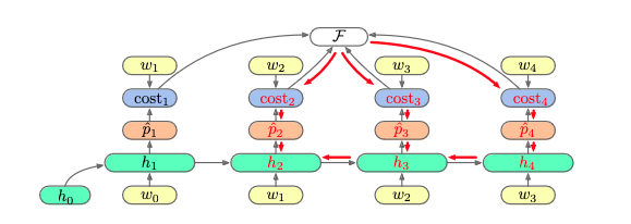
Can you state how the value of
\(\frac{\partial \mathcal F}{\partial \mathbf h _ 2}\)
would be calculated, and also state the general recursion used for calculating derivatives in reverse-mode differentiation like this?
In general, if we want to find the derivative of $\mathcal F$ with respect to a variable $v _ i$, we have the recurrence \(\sum _ {j : \text{ child of }v _ i \text{ in comp. graph} } \frac{\partial \mathcal F}{\partial v _ j} \frac{\partial v _ j}{\partial v _ i}\) then we can compute $\partial v _ j / \partial v _ i$ similarly.
(this is a “generalisation” of the chain rule)
Suppose we are training an RNN.
Unrolling the computational graph, we get the expression $\mathcal F = \sum _ n \mathcal F _ n$ for the loss. The goal of BPTT is to compute $\nabla _ \theta \mathcal F$, where $\theta$ are the parameters of the RNN. Letting $\theta _ n$ be the copy of the RNN parameters at timestep $n$ in the computational graph, $\nabla _ \theta$ is the sum of the gradients for each copy $\theta _ n$.
What is the general expression for how the gradients are calculated in BPTT?
We use the recurrence
\[\nabla _ \theta \mathcal F = \sum^N _ {n = 1} \frac{\partial F}{\partial \mathbf h _ n} \frac{\partial \mathbf h _ n}{\partial \theta _ n} = \sum^N _ {i = 1} \left[ \frac{\partial \mathcal F}{\partial \mathbf h _ {n+1} } \frac{\partial \mathbf h _ {n+1} }{\partial \mathbf h _ n} + \frac{\partial \mathcal F _ n}{\partial \mathbf h _ n} \right] \frac{\partial \mathbf h _ n}{\partial \theta _ n}\]Suppose we are training an RNN.
Unrolling the computational graph, we get the expression $\mathcal F = \sum _ n \mathcal F _ n$ for the loss. The goal of BPTT is to compute $\nabla _ \theta \mathcal F$, where $\theta$ are the parameters of the RNN. Letting $\theta _ n$ be the copy of the RNN parameters at timestep $n$ in the computational graph, $\nabla _ \theta$ is the sum of the gradients for each copy $\theta _ n$.
What is the general expression for how the gradients are calculated in RTRL where we use the forward mode of automatic differentiation rather than the backward mode?
We use the recurrence \(\nabla _ \theta \mathcal F = \sum^N _ {n = 1} \frac{\partial F}{\partial \mathbf h _ n} \frac{\partial \mathbf h _ n}{\partial \theta} = \sum^N _ {i = 1} \frac{\partial \mathcal F _ n}{\partial \pmb h _ n} \left[ \frac{\partial \pmb h _ n}{\partial \theta _ n } + \frac{\partial \pmb h _ n }{\partial \mathbf h _ {n-1} }\frac{\partial \mathbf h _ {n-1} }{\partial \theta} \right]\)