Lecture - Uncertainty in Deep Learning MT25, Uncertainty over functions

[[Course - Uncertainty in Deep Learning MT25]]^U
- Previous lecture: [[Lecture - Uncertainty in Deep Learning MT25, Bayesian probabilistic modelling of functions]]^U
- Next lecture: [[Lecture - Uncertainty in Deep Learning MT25, Approximate inference]]^U

In this lecture, we interpret the variance of the predictive distribution as splitting into the aleatoric uncertainty and the epistemic uncertainty.

Decomposing predictive uncertainty

Suppose:

We are consider a deep neural network with scalar outputs $y$
$W \in \mathbb R^{K \times 1}$ is the weight matrix of the last layer
$b = 0$ for the output layer
We don’t consider the rest of the weights of the network, so that we may write $f^W(\pmb x) = \sum w _ k \phi _ k(\pmb x) = W^\top \phi(\pmb x)$, where $\phi(\pmb x)$ is the feature map implemented by the previous layers of the network

and consider the following generative story:

Nature chose $W$ which defines a function $f^W(\pmb x)$ := W^\top \phi(x)$
Then nature generated function values with inputs $x _ 1, \ldots, x _ N$ given by $f^W(x _ n)$
These were corrupted with additive Gaussian noise $y _ n := f^W(x _ n) + \epsilon _ n$, $\epsilon _ n \sim \mathcal N(0, \sigma^2)$
We then observe these corrupted values ${(x _ 1, y _ 1), \ldots, (x _ N, y _ N)}$

Recall that this means we have:

Prior: $\mathbb P(w _ k) = \mathcal N(w _ k; 0, s^2)$
Likelihood: $\mathbb P(Y \mid W, X) = \prod _ n \mathcal N(y \mid W^\top \phi(x), \sigma^2)$
Posterior: $\mathbb P(W \mid X, Y) = \mathcal N(W \mid \mu’, \Sigma’)$, where:
- $\Sigma’ = (\sigma^{-2} \phi(X)^\top \phi(X) + s^{-2} I _ k)^{-1}$
- $\mu’ = \Sigma’ \sigma^{-2} \phi(X)^\top Y$
Predictive: $\mathbb P(y^\ast \mid x^\ast, X, Y) = \mathcal N (y^\ast \mid \mu^\ast, \sigma^\ast)$, where:
- $\sigma^\ast = \sigma^2 + \phi(x^\ast)^\top \Sigma’ \phi(x^\ast)$
- $\mu^\ast$: $(\mu’)^\top \phi(x^\ast)$

How can you interpret the predictive uncertainty $\sigma^\ast$?

Decompose it into

\[\underbrace{\sigma^2} _ \text{aleatoric uncertainty} + \underbrace{\phi(x^\ast) \Sigma' \phi(x^\ast)} _ \text{epistemic uncertainty}\]

Suppose:

We are consider a deep neural network with scalar outputs $y$
$W \in \mathbb R^{K \times 1}$ is the weight matrix of the last layer
$b = 0$ for the output layer
We don’t consider the rest of the weights of the network, so that we may write $f^W(\pmb x) = \sum w _ k \phi _ k(\pmb x) = W^\top \phi(\pmb x)$, where $\phi(\pmb x)$ is the feature map implemented by the previous layers of the network

and consider the following generative story:

Nature chose $W$ which defines a function $f^W(\pmb x)$ := W^\top \phi(x)$
Then nature generated function values with inputs $x _ 1, \ldots, x _ N$ given by $f^W(x _ n)$
These were corrupted with additive Gaussian noise $y _ n := f^W(x _ n) + \epsilon _ n$, $\epsilon _ n \sim \mathcal N(0, \sigma^2)$
We then observe these corrupted values ${(x _ 1, y _ 1), \ldots, (x _ N, y _ N)}$

Recall that this means we have:

Prior: $\mathbb P(w _ k) = \mathcal N(w _ k; 0, s^2)$
Likelihood: $\mathbb P(Y \mid W, X) = \prod _ n \mathcal N(y \mid W^\top \phi(x), \sigma^2)$
Posterior: $\mathbb P(W \mid X, Y) = \mathcal N(W \mid \mu’, \Sigma’)$, where:
- $\Sigma’ = (\sigma^{-2} \phi(X)^\top \phi(X) + s^{-2} I _ k)^{-1}$
- $\mu’ = \Sigma’ \sigma^{-2} \phi(X)^\top Y$
Predictive: $\mathbb P(y^\ast \mid x^\ast, X, Y) = \mathcal N (y^\ast \mid \mu^\ast, \sigma^\ast)$, where:
- $\sigma^\ast = \sigma^2 + \phi(x^\ast)^\top \Sigma’ \phi(x^\ast)$
- $\mu^\ast$: $(\mu’)^\top \phi(x^\ast)$

Recall that you can decompose the predictive variance into two terms

\[\underbrace{\sigma^2} _ \text{aleatoric uncertainty} + \underbrace{\phi(x^\ast) \Sigma' \phi(x^\ast)} _ \text{epistemic uncertainty}\]

How could you re-frame the generative story for this data to make this distinction between the aleatoric uncertainty and the epistemic uncertainty more clear?

@Prove that you can recover the aleatoric uncertainty and epistemic uncertainty separately under this new generative story by taking the variance over different conditions.

The initial generative story looks like this:

.png)

If we insert a new intermediate latent variable $f _ n$ which represents $W^\top \phi(x _ n)$ before it is corrupted with noise, we have:

.png)

Mathematically, we can represent this with a Dirac delta distribution:

\[\begin{aligned} &f _ n \mid x _ n, W \sim \delta(f _ n = W^\top \phi(x _ n)) \\ &y _ n \mid f _ n \sim \mathcal N(y _ n \mid f _ n, \sigma^2) \end{aligned}\]

The overall joint distribution over $W, x _ n, y _ n$ is the same, but now we have an extra variable that we can condition over. The interesting result is as follows:

\[\begin{aligned} &\text{Var} _ {\mathbb P(y^\ast \mid f^\ast, X, Y)}[y^\ast] = \sigma^2 \\ &\text{Var} _ {\mathbb P(f^\ast \mid x^\ast, X, Y)} [f^\ast] = \phi(x^\ast)^\top \Sigma' \phi(x^\ast) \end{aligned}\]

This demonstrates that the epistemic uncertainty term really is the epistemic uncertainty in what we believe the model parameters are, and the aleatoric uncertainty really is the inherent noise in the corrupted data.

To see $\text{Var} _ {\mathbb P(y^\ast \mid f^\ast, X, Y)}[y^\ast] = \sigma^2$, note that by the assumptions $y^\ast$ conditioned on $f^\ast$ is now independent of $X$ and $Y$. Therefore $\mathbb P(y^\ast \mid f^\ast, X, Y) = \mathbb P(y^\ast \mid f^\ast)$, and so since $y _ n \mid f _ n \sim \mathcal N(y _ n \mid f _ n, \sigma^2)$, it follows that

\[\text{Var} _ {\mathbb P(y^\ast \mid f^\ast, X, Y)} (y^\ast) = \text{Var} _ {\mathbb P(y^\ast \mid f^\ast)}(y^\ast) = \sigma^2 \\\]

Seeing the other inequality is a bit more involved:

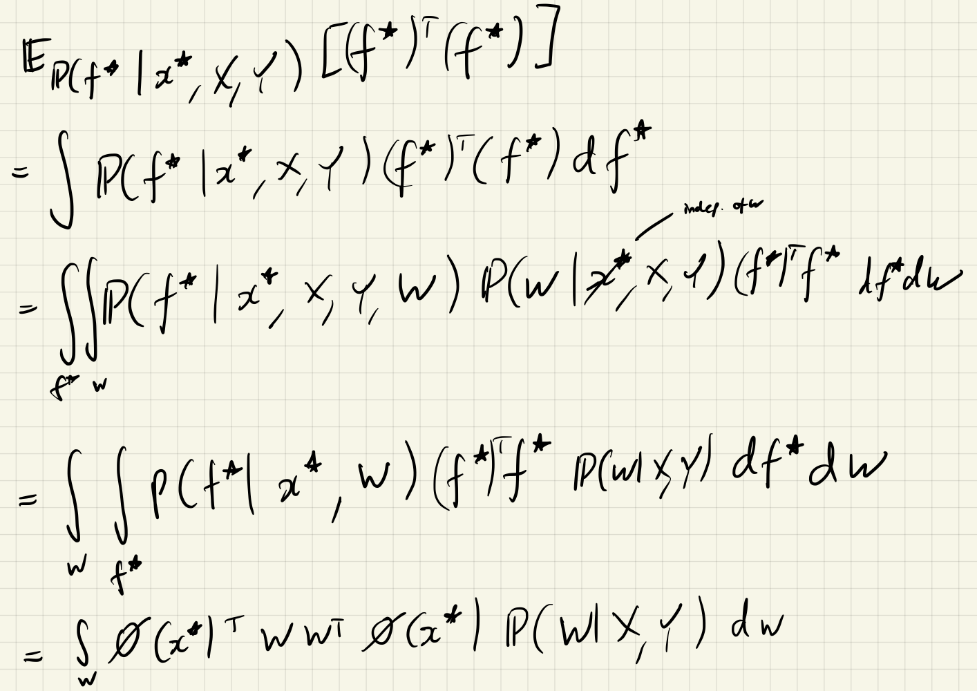
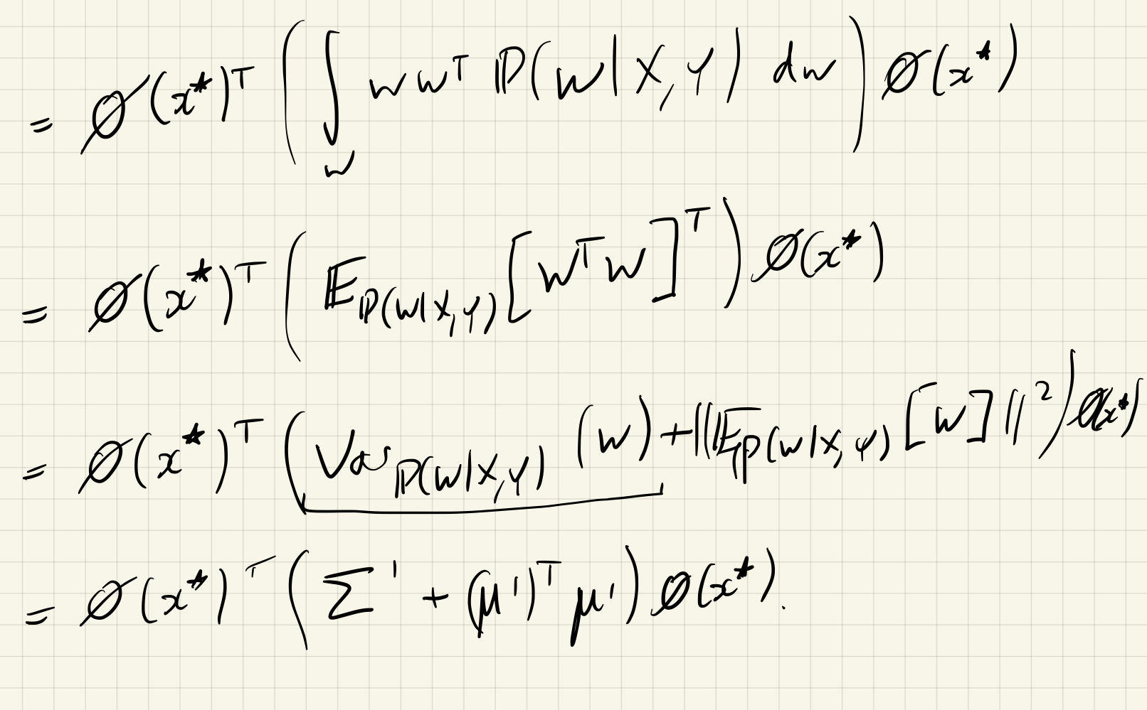
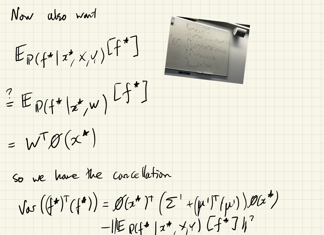
(there is a minor mistake somewhere here involving transposes…)

How well does the epistemic uncertainty term really capture epistemic uncertainty?

Suppose:

We are consider a deep neural network with scalar outputs $y$
$W \in \mathbb R^{K \times 1}$ is the weight matrix of the last layer
$b = 0$ for the output layer
We don’t consider the rest of the weights of the network, so that we may write $f^W(\pmb x) = \sum w _ k \phi _ k(\pmb x) = W^\top \phi(\pmb x)$, where $\phi(\pmb x)$ is the feature map implemented by the previous layers of the network

and consider the following generative story:

Nature chose $W$ which defines a function $f^W(\pmb x)$ := W^\top \phi(x)$
Then nature generated function values with inputs $x _ 1, \ldots, x _ N$ given by $f^W(x _ n)$
These were corrupted with additive Gaussian noise $y _ n := f^W(x _ n) + \epsilon _ n$, $\epsilon _ n \sim \mathcal N(0, \sigma^2)$
We then observe these corrupted values ${(x _ 1, y _ 1), \ldots, (x _ N, y _ N)}$

Recall that this means we have:

Prior: $\mathbb P(w _ k) = \mathcal N(w _ k; 0, s^2)$
Likelihood: $\mathbb P(Y \mid W, X) = \prod _ n \mathcal N(y \mid W^\top \phi(x), \sigma^2)$
Posterior: $\mathbb P(W \mid X, Y) = \mathcal N(W \mid \mu’, \Sigma’)$, where:
- $\Sigma’ = (\sigma^{-2} \phi(X)^\top \phi(X) + s^{-2} I _ k)^{-1}$
- $\mu’ = \Sigma’ \sigma^{-2} \phi(X)^\top Y$
Predictive: $\mathbb P(y^\ast \mid x^\ast, X, Y) = \mathcal N (y^\ast \mid \mu^\ast, \sigma^\ast)$, where:
- $\sigma^\ast = \sigma^2 + \phi(x^\ast)^\top \Sigma’ \phi(x^\ast)$
- $\mu^\ast$: $(\mu’)^\top \phi(x^\ast)$

We may decompose the predictive variance into two components:

\[\underbrace{\sigma^2} _ \text{aleatoric uncertainty} + \underbrace{\phi(x^\ast) \Sigma' \phi(x^\ast)} _ \text{epistemic uncertainty}\]

Let

\[\mathcal U(x^\ast) := \phi(x^\ast)^\top \Sigma' \phi(x^\ast)\]

@State some (informal, but possible to formalise) results about the behaviour of $\mathcal U(x^\ast)$.

$U(x^\ast) \gg 0$ when $x^\ast$ is dissimilar to the training data
$U(x^\ast) \approx 0$ when $x^\ast$ is similar to training data

…the lecturer plans to return the proof if there is time at the end of the course, since it’s quite long and quite involved…

Decomposing predictive uncertainty

How well does the epistemic uncertainty term really capture epistemic uncertainty?

Related posts