Computer Vision MT25, Convolutional neural networks
Flashcards
What was the “neocognitron”?
An early (Fukushima 1980) example of an image-processing neural network, trained layerwise using a method called “self-organising maps”.
What idea motivated CNNs?
They should be invariant to shifts, scale and small distortions.
What three properties of a CNN help make them learn to be invariant to shifts, scale and small distortions?
- Local weighted connections
- Shared weights across spatial locations
- Spatial subsampling
How are CNN architectures generally composed?
- Filters arranged with a width, height and depth
- Alternating convolutional and subsampling layers
- Fully connected layers at the end
What was maybe unnecessary about the filters used in LeNet?
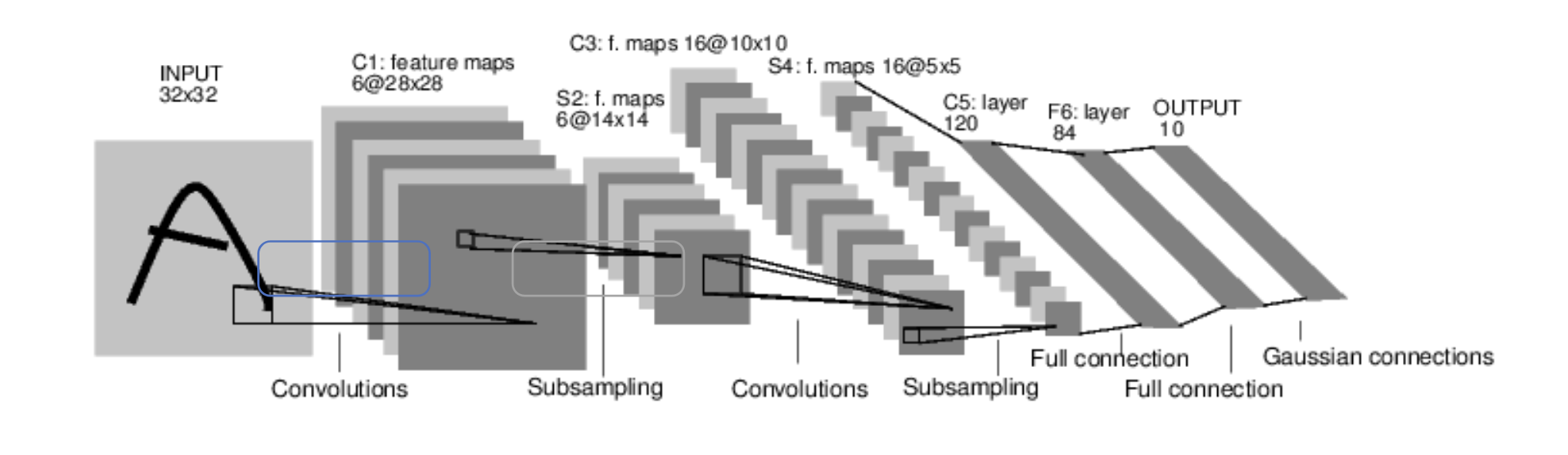
They were unnecessarily large, many later architectures used much smaller filters.
Suppose you have a convolutional filter of dimensions $h \times w \times d$. How much should you zero-pad the input?
Add $(h-1)/2$ cells to the top and bottom, and $(w-1)/2$ cells to the left and right.
Suppose you have a $10 \times 10 \times 3$ input volume, which you process by applying a $3 \times 3 \times 3$ convolutional filter with stride $1$ and zero-padding of $1$ on each side. What is the size of the resulting output volume?
Suppose:
- You have an input volume of size $h _ \text{in} \times w _ \text{in} \times d$
- You have a convolutional filter of size $h \times w \times d$ (although $d$ being the same here is not necessary)
- The stride of this filter is $s$
- Zero-padding of $p$ pixels is added on each side of the input
@State the dimensions of the output.
where
\[\begin{aligned} h _ \text{out} &= \frac{h _ \text{in} - h + 2p}{s} + 1 \\ w _ \text{out} &= \frac{w _ \text{in} - w + 2p}{s} + 1 \end{aligned}\]What are the hyperparameters of a convolution layer in a CNN?
- The number of filters
- The width and height of the filters
- The stride of each of the filters
- How padding is calculated
How is bias added in a convolutional layer of a CNN?
There is one scalar bias per filter, added uniformly to every spatial position of that filter’s output channel. So if the layer has $K$ filters, there are $K$ biases, and the output volume is $h _ \text{out} \times w _ \text{out} \times K$ where channel $k$ has the scalar $b _ k$ added to every entry.
Suppose:
- You have an input volume of size $h _ \text{in} \times w _ \text{in} \times d$
- You have a pooling layer of width $w$ and height $h$
- The stride is $s$
When does overlapping of the sliding window occur?
If $s < w$ or $s < h$.
Suppose:
- You have an input volume of size $h _ \text{in} \times w _ \text{in} \times d$
- You have a pooling layer of width $w$ and height $h$
- The stride is $s$
@State the dimensions of the output.
(pooling preserves the channel dimension, since it is applied independently to each channel) where
\[\begin{aligned} h _ \text{out} &= \frac{h _ \text{in} - h}{s} + 1 \\ w _ \text{out} &= \frac{w _ \text{in} - w}{s} + 1 \end{aligned}\]How can you interpret a fully connected layer as a convolutional layer?
Each filter has the same size as the input, so you can do an arbitrary linear combination of all the previous layers.
What was AlexNet, and what does its first-layer filter visualisation show?
AlexNet was an ImageNet winner that was the first to really try a deep learning approach. It did this using ReLU, GPU training, dropout and depth.

Its first layer filter visualisation showed it learned basic visual elements.

What was ResNet?
ResNet was a CNN that proposed the idea of skip/residual connections, and achieved state-of-the-art performance at the time.

The receptive field of a neuron in a CNN is the region of the input image whose values can affect that neuron’s activation. For a stack of conv layers, the receptive field grows with depth, but exactly how depends on each layer’s kernel size and stride.
Suppose we define for each layer $\ell$:
- $r _ \ell$: the receptive field size (in input pixels), after layer $\ell$
- $j _ \ell$: the cumulative jump after layer $\ell$, i.e. how many input pixels you skip when you move one cell in layer $\ell$’s output feature map.
- $k _ \ell, s _ \ell$: kernel size and stride of layer $\ell$
@State the initial values for $r _ 0$ and $j _ 0$ and a recurrence relating $r _ \ell$ and $j _ \ell$ to the previous layer.
Initial values (the input layer itself — every “neuron” is one pixel, and adjacent neurons are one pixel apart):
\[r _ 0 = 1, \quad j _ 0 = 1.\]Recurrence for $\ell \ge 1$:
\[r _ \ell = r _ {\ell - 1} + (k _ \ell - 1) j _ {\ell - 1}, \quad j _ \ell = j _ {\ell-1} \, s _ \ell.\]Bite-sized
The ReLU activation is $f(x) = <span class="cloze" tabindex="0">\max(0, x)</span>$. It is computationally cheap, non-saturating for $x > 0$ (gradient $1$), and produces a sparse activation pattern (gradient $0$ for $x < 0$).
@Justify why ReLU is generally preferred over sigmoid or tanh activations in deep networks.
- No saturation for $x > 0$: ReLU’s gradient is $1$ for positive inputs, so signals propagate cleanly through deep stacks. Sigmoid/tanh saturate at both ends, where their derivative is close to zero — the vanishing gradient problem that prevents deep networks from training.
- Sparse activation: ReLU outputs exact zeros for negative pre-activations, so only a subset of neurons fire on each input. This can improve representation and conditioning.
- Computational efficiency: a simple thresholding compared to evaluating $1/(1+e^{-x})$ or $\tanh$.
SGD with momentum updates the weights as $\Delta w _ t = <span class="cloze" tabindex="0">\rho \Delta w _ {t-1} - \lambda g _ t</span>$, where $\rho$ is the momentum coefficient, $\lambda$ is the learning rate and $g _ t$ is the current mini-batch gradient. The momentum accelerates progress when the gradient direction is consistent and dampens oscillations across narrow valleys.
@State the four equations defining the Adam optimiser (first moment, second moment, bias correction, parameter update).
For mini-batch gradient $g _ t$, with hyperparameters $\beta _ 1 = 0.9$, $\beta _ 2 = 0.999$, learning rate $\lambda$, and stabiliser $\varepsilon$:
- First moment (mean): $m _ t = \beta _ 1 m _ {t-1} + (1 - \beta _ 1) g _ t$
- Second moment (uncentred variance): $v _ t = \beta _ 2 v _ {t-1} + (1 - \beta _ 2) g _ t^2$
- Bias correction: $\hat m _ t = m _ t / (1 - \beta _ 1^t)$, $\hat v _ t = v _ t / (1 - \beta _ 2^t)$
- Update: $\Delta w _ t = -\dfrac{\lambda}{\sqrt{\hat v _ t} + \varepsilon} \, \hat m _ t$
Bias correction is needed because $m _ 0 = v _ 0 = 0$ otherwise pulls the early-step estimates toward zero.
$L _ 2$ regularisation adds the penalty $R = <span class="cloze" tabindex="0">\tfrac{1}{2} \alpha w^2</span>$ to the loss; $L _ 1$ regularisation adds the penalty $R = <span class="cloze" tabindex="0">\alpha \vert w \vert</span>$. $L _ 2$ keeps weights small and diffuse (linear decay in the gradient update), while $L _ 1$ encourages sparse weights (many exactly zero).
The activation function family covered in the lecture includes sigmoid, tanh, ReLU, Parametric ReLU (PReLU), Leaky ReLU, SELU, ELU, GELU, and Swish. They differ in saturation behaviour, smoothness, treatment of negative inputs (zeroing, leaking, exponential, gated), and whether they’re parameter-free.
The first convolutional layer of AlexNet (Krizhevsky, Sutskever, Hinton, NeurIPS 2012) has 96 filters of size $11 \times 11 \times 3$. Visualising these filters reveals oriented edge detectors, blobs, and colour-opponent patterns reminiscent of biological V1 cells.

The popular ResNet variants discussed in the lecture are R18, R50, R101, R152 (suffix = depth in layers), all built from the same residual block primitive but at increasing depth.
@Justify why a non-linearity (e.g. ReLU) is inserted between successive convolution layers in a CNN.
Convolution is a linear operation. The composition of two linear operators is itself a single linear operator, so stacking convs without a non-linearity collapses the entire network into a single (equivalent) linear function and the depth gains no representational power.
Inserting a non-linearity between conv layers breaks this collapse, giving the network the ability to model non-linear input-output mappings.
Pooling provides invariance to small spatial shifts of the input (because precise spatial location within the pooling window is discarded), and also reduces spatial resolution (cheap subsampling) without learnable parameters.
In a $K$-filter convolutional layer applied to a $d$-channel input, each filter has spatial size $h \times w$ and depth equal to the input depth $d$. Thus a single filter contains $h \cdot w \cdot d$ weights, plus 1 bias, giving the full layer $K \cdot (h \cdot w \cdot d + 1)$ learnable parameters total.
LeNet-5 was introduced by LeCun et al. in 1998 for handwritten digit recognition, was the first successful modern CNN architecture, and was trained end-to-end with back-propagation and gradient descent.
Visualising the receptive field
The recurrence ∆receptive-field-recurrence is easiest to feel by tracing a single output neuron back to the input pixels that can reach it. Add or remove convolutional layers, change each layer’s kernel size and stride, and click any output neuron to watch its receptive field grow on the input.
