Computer Vision MT25, Neural networks
Flashcards
Residual connections
One part of a neural network could be interpreted as calculating
\[y = f(x)\]
With residual connections, you instead calculate
\[y = f(x) + x\]
Can you give some intuition for why this might be easier to train?
- In the first option, the network needs to learn to pass on all the information in $x$ to the following layer.
- In the second option, the network only needs to learn the changes in the representation $f(x) = y - x$.
- This means gradients flow much easier through the network.
Batch normalisation
Consider a single layer with ReLU
\[y = \max(0, Wx + b)\]
After initialisation, $W$ and $b$ can be hard to learn (e.g. if $x$ is small, then $W$ needs to be large, and if $x$ is negative, $b$ needs to large to avoid $0$ gradient from ReLU).
Given $x \in \mathbb R^{B \times d}$, how does batch normalisation solve some of these problems, and what is $y \in \mathbb R^{B \times d}$?
We use the batch statistics in order to normalise the outputs of layers, so that the inputs $x$ are “well-behaved” for optimisation, calculating $y = \text{BN}(x) \in \mathbb R^{B \times d}$ where:
- $y _ {i, j} = \gamma _ j x _ {i,j}’ + \beta _ j$, where $\gamma, \beta$ are learnt
- $x _ {i, j}’ = \frac{1}{\sigma^2 _ j + \epsilon} (x _ {i, j} - \mu _ j)$
- $\sigma^2 = \frac 1 B \sum^B _ {i = 1} (x _ i - \mu)^2 \in \mathbb R^d$
- $\mu = \frac{1}{B} \sum^B _ {i = 1} x _ i \in \mathbb R^d$
After batch normalisation, what do you expect to be true about 50% of activations in a ReLU network?
They are $0$.
Where does batch normalisation typically go in a neural network?
After fully connected or convolution layers, and before nonlinearities.
Why can batch normalisation be a large source of bugs?
It behaves differently during training and testing.
Batch normalisation requires statistics to be computed from batches of the input data. How are these statistics found at test time?
They are fixed.
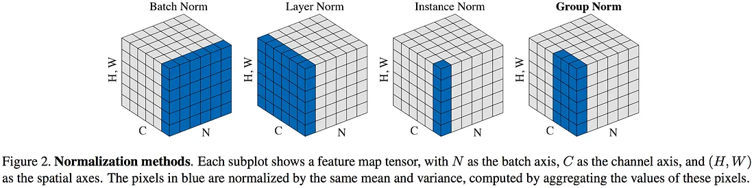
@Visualise the difference between:
- Batch norm
- Layer norm
- Instance norm
- Group norm
Transfer learning
What is transfer learning?
You train a some model on a large dataset for some related task, and then fine-tune on your task that has less data.
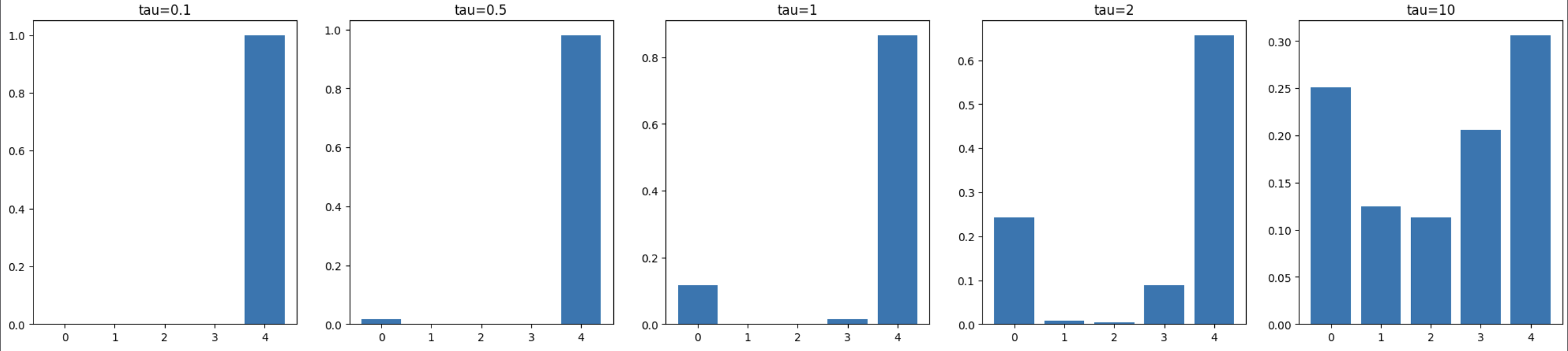
Softmax and temperature
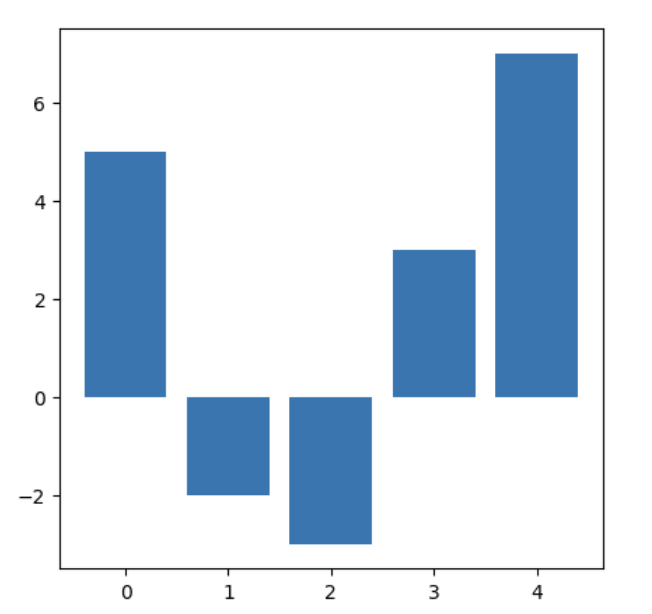
@Define the $\text{softmax}(Y, \tau)$ with temperature function, @state three results that intuitively relate it to just taking the argmax of some set of predictions, and @visualise how varying $\tau$ affects the distribution derived from the following input data:
.
where $\hat Y$ is the vector of predictions for each class. We have the results that:
- It maintains the relative ordering: $\text{softmax} _ i(\hat Y, \tau _ 1) < \text{softmax} _ j(\hat Y, \tau _ 1) \implies \text{softmax} _ i(\hat Y, \tau _ 2) < \text{softmax} _ j(\hat Y, \tau _ 2)$
- As $\tau \to \infty$, softmax becomes a uniform distribution.
- As $\tau \to 0$, softmax becomes argmax (as one-hot).