Computer Vision MT25, Fourier transform
Flashcards
1D case
@Define the Fourier transform of a function $f : \mathbb R \to \mathbb R$, and the inverse Fourier transform.
(where $\psi _ u(t) = e^{i2\pi u t}$).
In Fourier analysis, a function $f : \mathbb R \to \mathbb R$ is written as a weighted combination of orthonormal basis functions $\psi _ u (t)$. @Define $\psi _ u (t)$. With respect to which inner product are they orthonormal?
where $u \in (-\infty, \infty)$. They are orthonormal with respect to
\[\langle g, h \rangle = \int^\infty _ {-\infty} g(t) h^\ast (t) \text dt\]@Describe how you can interpret the Fourier transform as letting you write a function $f : \mathbb R \to \mathbb R$ as a weighted “sum” of basis functions.
The inverse Fourier transform says that you can write
\[f(t) = \int^\infty _ {-\infty} F(u) e^{i2\pi u t} \text du\]In this way, $f$ is a weighted combination of basis functions $e^{i 2\pi u t}$.
The Fourier transform associates with a function $f : \mathbb R \to \mathbb R$ a function
\[F(u) = \int^\infty _ {-\infty} f(t) e^{-i2\pi u t} \text dt = \langle f, \psi _ u \rangle\]
such that
\[f(t) = \int^\infty _ {-\infty} F(u) e^{i 2\pi u t} \text du\]
where $\psi _ u(t) = e^{i2\pi u t}$. Interpreting $F(u)$ weights corresponding to sinusoids
\[A \sin(2\pi u t + \phi)\]
in the decomposition of $f(t)$, what is the amplitude $A$ and phase $\phi$ in terms of $F(u)$?
The Fourier transform associates with a function $f : \mathbb R \to \mathbb R$ a function
\[F(u) = \int^\infty _ {-\infty} f(t) e^{-i2\pi u t} \text dt = \langle f, \psi _ u \rangle\]
such that
\[f(t) = \int^\infty _ {-\infty} F(u) e^{i 2\pi u t} \text du\]
where $\psi _ u(t) = e^{i2\pi u t}$. When $f(t)$ is real, what useful identities are there surrounding the real and imaginary parts of $F$?
- $\Re(F(u)) = \Re(F(-u))$
- $\Im(F(u)) = -\Im(F(-u))$ (this is why undoing the Fourier transform doesn’t introduce complex values)
@Define the discrete Fourier transform of a function $f : {0, 1, \ldots, N-1} \to \mathbb R$, and the inverse discrete Fourier transform.
(where $\psi _ k(t) = e^{i\frac{2\pi k}{N} n}$).
The discrete Fourier transform of a function $f : {0, 1, \ldots, N-1} \to \mathbb R$, and the inverse discrete Fourier transform are given by
\[\begin{aligned}
F(k) &= \sum^{N-1} _ {n = 0} f(n) e^{-i \frac{2\pi k}{N}n} = \langle f, \psi _ k \rangle \\
f(n) &= \frac{1}{N} \sum^{N-1} _ {n = 0} f(n) e^{i \frac{2\pi k}{N}n}
\end{aligned}\]
where $\psi _ k(t) = e^{i\frac{2\pi k}{N} n}$. How could compute these via matrix-vector multiplications?
Consider $f$ as a vector in $\mathbb R^N$. Then $F$ is a vector in $\mathbb C^N$ given by
\[F = Uf\]where $U _ {k,n} := e^{-i 2\pi k n / N}$, and
\[f = U^{-1} F = \frac 1 N U^\ast F\]The discrete Fourier transform of a function $f : {0, 1, \ldots, N-1} \to \mathbb R$, and the inverse discrete Fourier transform are given by
\[\begin{aligned}
F(k) &= \sum^{N-1} _ {n = 0} f(n) e^{-i \frac{2\pi k}{N}n} = \langle f, \psi _ k \rangle \\
f(n) &= \frac{1}{N} \sum^{N-1} _ {n = 0} f(n) e^{i \frac{2\pi k}{N}n}
\end{aligned}\]
where $\psi _ k(t) = e^{i\frac{2\pi k}{N} n}$. What is always true about $F(k)$ and the result of any inverse DFT?
It is always periodic.
2D case
@Define the 2D Fourier basis function $\psi _ {u, v} (x, y)$.
@Visualise what the real parts of the 2D Fourier basis functions
\[\psi _ {u, v}(x, y) = e^{i 2\pi (ux + vy)}\]
look like for increasing values of $u$ and $v$.
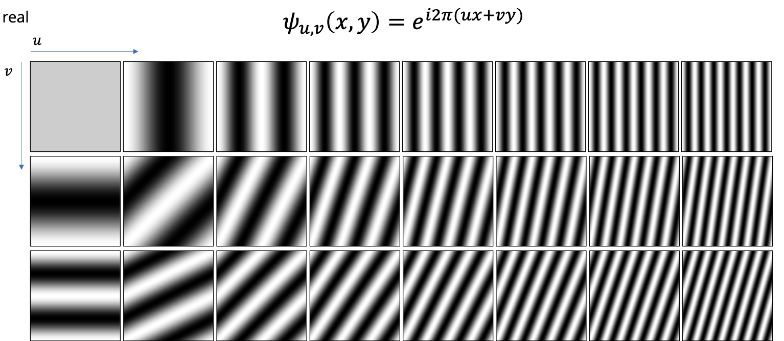
What are plots of the 2D Fourier transform like the following are actually showing?
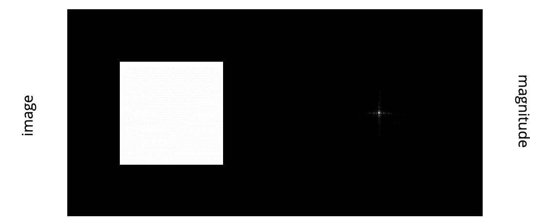
On the left is the original image, on the right is the plot of the magnitude of the Fourier coefficients $\psi _ {u, v}(x, y) = e^{i 2\pi (ux + vy)}$.
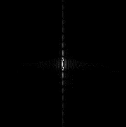
What does the following image look like in the frequency domain?

@example~
What does the following image look like in the frequency domain?

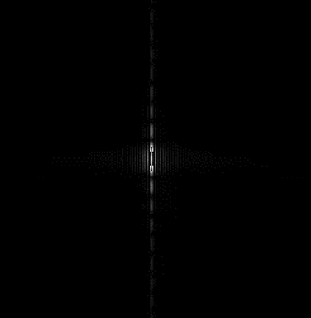
@example~
What does the following image look like in the frequency domain?
@example~
Convolution theorem
@State the convolution theorem.
The Fourier transform of the convolution of two functions is the (pointwise) product of their Fourier transforms:
\[\mathcal F\{ f\ast g \} = \mathcal F\{f\} \mathcal F\{g\}\]The inverse Fourier transform of the product of two Fourier transforms is the convolution of the two inverse Fourier transforms:
\[\mathcal F^{-1}\{FG\} = \mathcal F^{-1}\{F\} \ast \mathcal F^{-1}\{G\}\]The ∆convolution-theorem states that
The Fourier transform of the convolution of two functions is the product of their Fourier transforms:
\[\mathcal F\{ f\ast g \} = \mathcal F\{f\} \mathcal F\{g\}\]
The inverse Fourier transform of the product of two Fourier transforms is the convolution of the two inverse Fourier transforms:
\[\mathcal F^{-1}\{FG\} = \mathcal F^{-1}\{F\} \ast \mathcal F^{-1}\{G\}\]
How can this be used to speed up the calculation of a convolution $f \ast g$?
The Fourier transform of the convolution of two functions is the product of their Fourier transforms:
The inverse Fourier transform of the product of two Fourier transforms is the convolution of the two inverse Fourier transforms:
Computing $f \ast g$ in the spatial domain is $O(N^2)$, but the complexity of computing $\mathcal F^{-1} { \mathcal F{f} \mathcal F{g} }$ is $O(N \log N)$ using the fast Fourier transform.
@State the time complexity of computing the DFT of a function $f : {0, 1, \ldots, N-1}$ and the IDFT of the corresponding $\mathcal F {f}$.
using the fast Fourier transform.
Filters using the Fourier transform
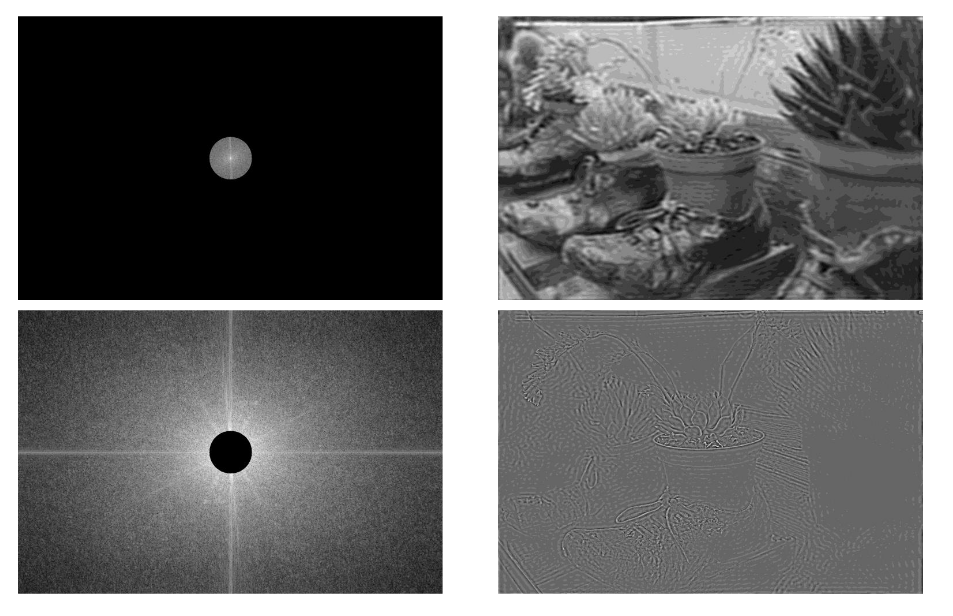
Explain and @visualise how you could implement a low- or high-pass filter on an image $f$.
Compute the DFT of the image $f$, remove the high or low frequencies, and then apply the IDFT.
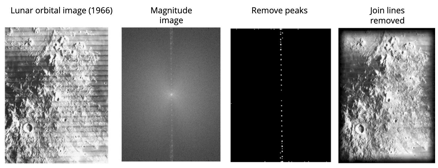
Explain and visualise how you could remove the periodic pattern in this image
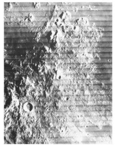
using the Fourier transform.
Calculate the DFT, remove the peaks, and then apply the IDFT.