Computer Vision MT25, Filtering
Flashcards
Suppose we are creating a new image $g$ from a source image $f$ by a filtering operation. The general setup is that
\[g(x, y) = F(N(x, y))\]
where $N$ is some neighbourhood of $(x, y)$. @Define a simple blur.
Suppose we are creating a new image $g$ from a source image $f$ by a filtering operation. The general setup is that
\[g(x, y) = F(N(x, y))\]
where $N$ is some neighbourhood of $(x, y)$. @Define a Gaussian blur.
where
\[w(u, v) = e^{-\frac{(x - u)^2 + (y-v)^2}{2\sigma^2}}\]Suppose we are creating a new image $g$ from a source image $f$ by a filtering operation. The general setup is that
\[g(x, y) = F(N(x, y))\]
where $N$ is some neighbourhood function. @Define a bilateral filter. What’s the intuition behind this?
where
\[\begin{aligned} w(u, v) &= w _ g(u, v) w _ s(u, v) \\ w _ g(u, v) &= e^{-\frac{(x - u)^2 + (y-v)^2}{2\sigma^2 _ g}} \\ w _ s(u, v) &= e^{-\frac{(f(u, v) - f(x, y))^2}{2\sigma^2 _ s}} \end{aligned}\]The intuition is that there are now two factors affecting how important a pixel is to the averaging operation:
- How close it is to the pixel under consideration
- How similar it is to the pixel under consideration
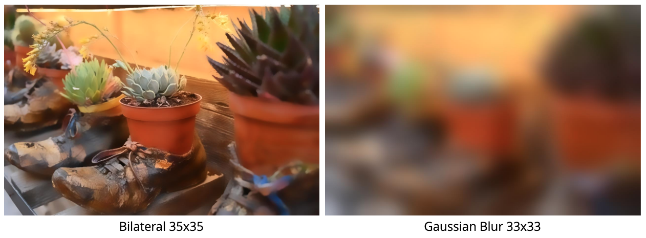
@Visualise the difference between a bilateral filter and a Gaussian filter applied to the same image.
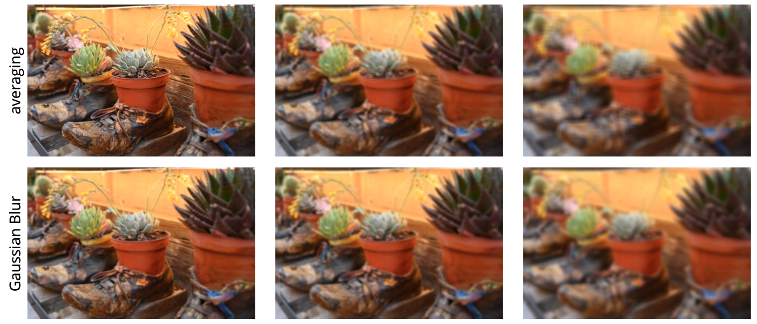
@Visuaslise the difference between an image filtered via a simple blur versus a Gaussian blur.
Suppose
What $f$ would be if $f \ast g$ corresponded to a $3 \times 3$ box blur?
@Visualise the effect of median filtering
\[F(N) = \text{median} _ {(u, v) \in N} \, f(u, v)\]
on an image. In what common circumstance is median filtering useful?
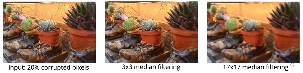
Median filtering is useful for outlier removal.
Bite-sized
@Justify why Gaussian blur is generally preferred over a box (mean) blur of the same size.
A box blur weights every pixel in the neighbourhood equally, which produces visible blocky artefacts (sharp transitions at the edges of the support region) and corresponds in the frequency domain to multiplication by a sinc with prominent sidelobes — these sidelobes cause ringing.
A Gaussian blur smoothly decays the weight $w(u,v) = e^{-((x-u)^2 + (y-v)^2)/(2\sigma^2)}$, so distant pixels contribute less than nearby pixels. The Fourier transform of a Gaussian is another Gaussian (no sidelobes), so Gaussian blur acts as a clean low-pass filter without ringing.
The result is a much more natural-looking blur for the same effective neighbourhood size.
Median filtering is a non-linear filter (it is not expressible as a convolution), and is particularly useful for removing salt-and-pepper noise or other impulse outliers — because the median is much less sensitive to outliers than the mean.
@Define the two scale parameters $\sigma _ g$ and $\sigma _ s$ in the bilateral filter and what each controls.
The bilateral weight $w(u,v) = w _ g(u,v)\, w _ s(u,v)$ is a product of two Gaussians:
- Spatial Gaussian $w _ g(u,v) = e^{-((x-u)^2 + (y-v)^2)/(2\sigma _ g^2)}$ controlled by $\sigma _ g$: how much spatially distant pixels contribute. Larger $\sigma _ g$ = stronger overall blur.
- Intensity Gaussian $w _ s(u,v) = e^{-(f(u,v) - f(x,y))^2/(2\sigma _ s^2)}$ controlled by $\sigma _ s$: how much pixels with dissimilar intensities contribute. Larger $\sigma _ s$ = more tolerant of intensity differences = bilateral acts more like a plain Gaussian blur. Small $\sigma _ s$ = strongly down-weights pixels across an edge, preserving the edge.
The interaction: $\sigma _ g$ controls extent, $\sigma _ s$ controls edge sensitivity — this is what gives the bilateral filter its edge-preserving smoothing behaviour.
The 2D isotropic Gaussian is separable: the kernel $G(x, y) = e^{-(x^2 + y^2)/(2\sigma^2)}$ factorises as $G _ 1(x) \cdot G _ 1(y)$ where $G _ 1$ is the 1D Gaussian. As a result, a 2D Gaussian blur of size $k \times k$ can be implemented as two successive 1D convolutions (one along each axis), reducing the per-pixel cost from $O(k^2)$ to $O(k)$.
@Describe the three categories of image transformation for an image considered as a function $f(x, y)$.
For an image regarded as a function $f(x, y)$, the three categories of transformation are:
- Point-wise transformation: $f'(x, y) = t(f(x, y))$ — operates on the range of the image. Examples: negation, contrast adjustment, gamma correction.
- Geometric transformation: $f'(x, y) = f(T(x, y))$ — operates on the domain of the image. Examples: translation, rotation, scaling, shearing, homography.
- Filtering: $f'(x, y) = F(N(x, y))$ for a neighbourhood $N(x, y)$ — operates on a local neighbourhood. Examples: blur, sharpen, median, bilateral.
This taxonomy is the organising frame for Lectures 2-3 and shows up again as a question in many problem sheets.
A simple box / mean blur with a $3 \times 3$ kernel is implemented as convolution with the kernel
\[f = \tfrac{1}{9} \begin{bmatrix} 1 & 1 & 1 \\ 1 & 1 & 1 \\ 1 & 1 & 1 \end{bmatrix}\]The normalising factor $\tfrac{1}{9}$ ensures $\sum f = <span class="cloze" tabindex="0">1</span>$, so the filter is energy-preserving (a constant input produces a constant output).