Computer Vision MT25, Neural rendering
Flashcards
The rendering equation
@State and @visualise the rendering equation for determining how much light $L _ o$ of wavelength $\lambda$ is leaving a point $x$ in the direction of $\omega _ 0$ at time $t$.
where $L _ e$ is the emitted radiance and $L _ r$ is the reflected radiance, defined by
\[L _ r(x, \omega _ 0, \lambda, t) = \int _ \Omega f _ r(x, \omega _ i, \omega _ o, \lambda, t) L _ i(x, \omega _ i, \lambda, t) (\omega _ i \cdot \pmb n) \text d\omega _ i\]and:
- $f _ r$ is the bidirectional reflectance distribution function (BRDF), which describes the intensity that the reflected light from direction $\omega _ i$ reflects to the observer
- $L _ i$ is the incoming radiance at $x$ from direction $\omega _ i$
- $\pmb n$ is the surface norm at $x$
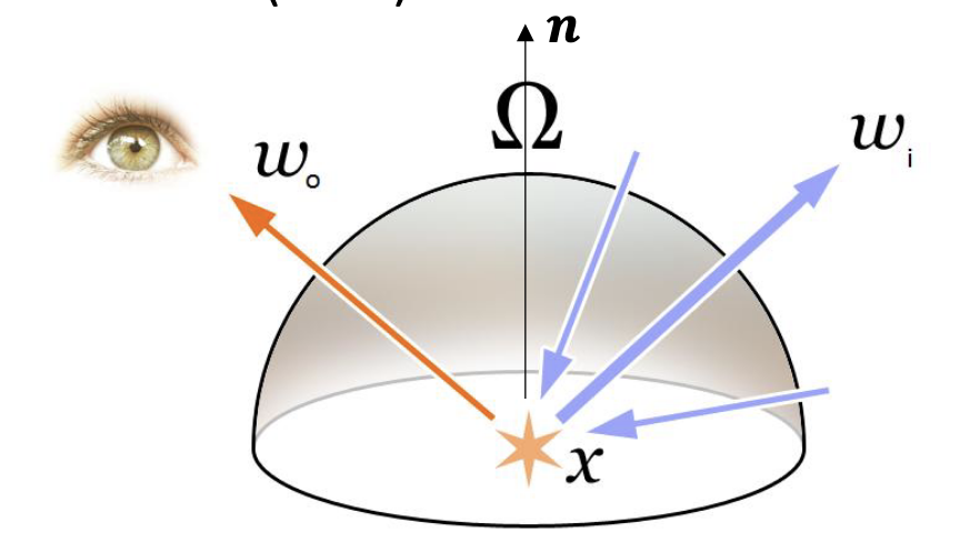
The rendering equation for determining how much light $L _ o$ of wavelength $\lambda$ is leaving a point $x$ in the direction of $\omega _ 0$ at time $t$ is given by
\[L _ o(x, \omega _ 0, \lambda, t) = L _ e(x, \omega _ o, \lambda, t) + L _ r(x, \omega _ o, \lambda, t)\]
where $L _ e$ is the emitted radiance and $L _ r$ is the reflected radiance, defined by
\[L _ r(x, \omega _ 0, \lambda, t) = \int _ \Omega f _ r(x, \omega _ i, \omega _ o, \lambda, t) L _ i(x, \omega _ i, \lambda, t) (\omega _ i \cdot \pmb n) \text d\omega _ i\]
and:
- $f _ r$ is the bidirectional reflectance distribution function (BRDF), which describes the intensity that the reflected light from direction $\omega _ i$ reflects to the observer
- $L _ i$ is the incoming radiance at $x$ from direction $\omega _ i$
- $\pmb n$ is the surface norm at $x$
@State the definition of $f _ r$ in terms of the $L _ r$ and the surface normal $\pmb n$, and state three properties that need to be true about any $f _ r$.
- Positivity: $f _ r(\omega _ i, \omega _ r) > 0$
- Reciprocity: $f _ r(\omega _ i, \omega _ r) = f _ r(\omega _ r, \omega _ i)$
- Energy conservation: $\forall \omega _ i, \int _ \Omega f _ r(\omega _ i, \omega _ r)(\omega _ r \cdot \pmb n) \text d\omega _ r \le 1$
Neural radiance fields
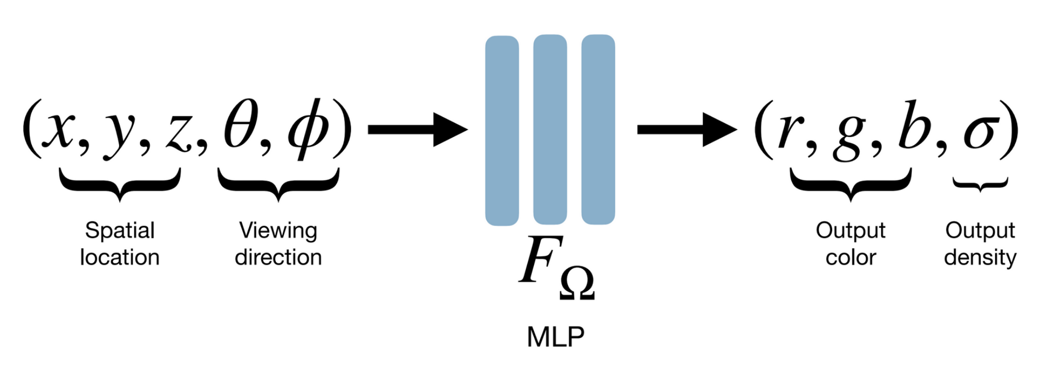
@State the typical problem setup in neural radiance fields.
- Input: Collection of images of some scene
- Learning: Mapping coordinates $(x, y, z, \theta, \phi)$ (3D position plus 2D viewing direction) to colour and density: $F _ \Omega : (x, y, z, \theta, \phi) \to (r, g, b, \sigma)$
- Output: Rendering of scene from new viewpoints
In neural radiance fields, the typical setup is:
- Input: Collection of images of some scene
- Learning: Mapping coordinates $(x, y, z, \theta, \phi)$ (3D position plus 2D viewing direction) to colour and density: $F _ \Omega : (x, y, z, \theta, \phi) \to (r, g, b, \sigma)$
- Output: Rendering of scene from new viewpoints
How is the loss determined?
We render an image using the model via direct volume rendering, and compare this to a ground truth image.
@State the equation used to determine the colour of a point corresponding to a ray emerging from the camera $r(t) = o + td$ when performing direct volume rendering.
where the sum is taken over some finite amount of steps along the ray, and:
- $T _ i$ is the visibility of that point, given by a product of previous opacities $T _ i = \prod^{i - 1} _ {j = 1}(1 - \alpha _ j)$
- $\alpha _ i$ is the opacity of a point, given by $\alpha _ i = 1 - e^{-\sigma _ i \Delta _ t}$
@Describe textual inversion for personalising text-to-image generation.
Goal: teach a pretrained text-to-image diffusion model a new visual concept (e.g. a specific teapot) from a few example images, so it can be references later via a new “word” $\langle e \rangle$.
Method:
- Introduce a placeholder token $\langle e \rangle$ into the model’s vocabulary
- Freeze everything else, so we only optimise for the embedding of $\langle e \rangle$
- Train by reconstruction: given example images of the target concept, condition the diffusion model on prompts like “an image of $\langle e \rangle$” and minimise the standard diffusion training loss against the example images.
@Describe how a diffusion model may be used as a prior for unsupervised 3D shape learning.
Goal: learn a 3D representation of an object from a text prompt alone or single photograph alone, with no multi-view photographs of that object as supervision.
Idea: instead of a multi-view ground truth, use a pretrained 2D diffusion model as the supervision signal. Either the diffusion has learned a “natural image” prior over the images matching the prompt, or textual inversion can be used to convert a single reference image to a text representation.
Pipeline: at each training step,
- Sample a camera pose
- Render the NeRF from that pose to produce an image
- Add noise to the rendered image
- Pass it through a frozen pretrained 2D diffusion model conditioned on the prompt, to denoise
- Compute MSE between the original rendered image and the denoised version, and backpropagate through the renderer to update the NeRF
View-conditioned prompts: in practice the prompt at each step is augmented with the sampled camera direction (e.g. “a picture of $\langle e \rangle$ from the side”), so the diffusion model’s gradient reflects the orientation being rendered. Without this, the diffusion prior places front-facing features on every side of the object (∆janus-problem). This view-conditioned prompting and ∆textual-inversion's $\langle e \rangle$ token are pieces of the same pipeline, not separate techniques.
@Define the Janus problem in diffusion-prior-based 3D reconstruction.
When using a 2D diffusion model as a prior for 3D shape learning (∆diffusion-as-prior-for-3d), the diffusion model is biased toward front-facing views. The optimised 3D reconstruction therefore tends to place front-facing features (e.g. faces) on every side of the object, like the two-faced Roman god Janus.

Bite-sized
NeRF was introduced by Mildenhall et al., ECCV 2020 in “NeRF: Representing scenes as neural radiance fields for view synthesis”. The architecture is an MLP $F _ \Omega: (x, y, z, \theta, \phi) \to (r, g, b, \sigma)$ that maps 5D spatial-plus-viewing-direction coordinates to colour and density.
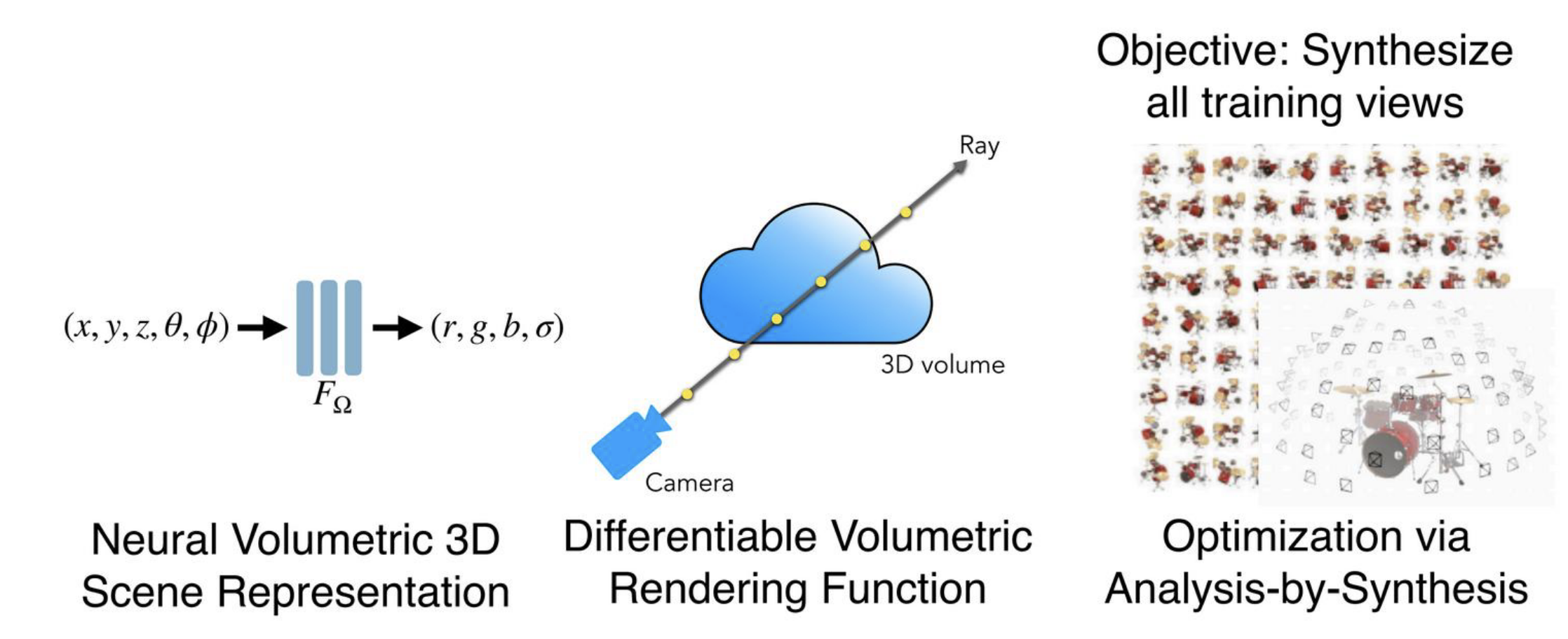
@State the three key components of NeRF and what each provides.
- Neural Volumetric 3D Scene Representation: an MLP $F _ \Omega(x, y, z, \theta, \phi) \to (r, g, b, \sigma)$ that stores the scene as a continuous function rather than a discrete voxel grid. Compact and queryable at any point/direction.
- Differentiable Volumetric Rendering: the volume rendering equation $C \approx \sum _ i T _ i \alpha _ i c _ i$ is differentiable in $\sigma _ i$ and $c _ i$, so we can backprop a per-pixel image loss through the rendering to update $F _ \Omega$.
- Optimisation via Analysis-by-Synthesis: the objective is simply to reproduce the input training views. No 3D supervision is needed — only multi-view 2D images and known camera poses (typically from COLMAP).
The opacity of a sample along a NeRF ray is given by $\alpha _ i = <span class="cloze" tabindex="0">1 - e^{-\sigma _ i \Delta t}</span>$ where $\sigma _ i$ is the predicted density at that point and $\Delta t$ is the step size along the ray. Higher density means higher opacity.
The transmittance up to sample $i$ along a NeRF ray is the cumulative product $T _ i = <span class="cloze" tabindex="0">\prod _ {j=1}^{i-1} (1 - \alpha _ j)</span>$ — the probability that the ray has not yet been absorbed by any earlier sample. The product index is $j$, not $i$ (a common transcription error to flag).
@Justify each of the three BRDF properties (positivity, reciprocity, energy conservation) in physical terms.
- Positivity $f _ r(\omega _ i, \omega _ r) > 0$: light cannot be reflected with negative intensity. A surface can absorb light (reflect zero) but cannot make a direction “darker than dark”.
- Reciprocity $f _ r(\omega _ i, \omega _ r) = f _ r(\omega _ r, \omega _ i)$ (Helmholtz reciprocity): swapping the roles of source and observer leaves the BRDF unchanged. Follows from time-reversal symmetry of EM and is what lets path-tracing renderers reverse rays from camera to light source.
- Energy conservation $\forall \omega _ i, \int _ \Omega f _ r(\omega _ i, \omega _ r)(\omega _ r \cdot \pmb n)\, d\omega _ r \le 1$: the total reflected energy cannot exceed the incoming energy. Equality corresponds to a perfectly lossless reflector; real materials have $< 1$ due to absorption.
Together these define a physically plausible BRDF, and rule out e.g. simple Phong shading (which violates reciprocity in its basic form).
3D Gaussian Splatting (Kerbl et al., SIGGRAPH 2023) is the modern alternative to NeRF. Instead of an MLP storing the scene, it represents the scene as a collection of 3D Gaussians (mean + covariance) projected to 2D Gaussians on the image plane. Advantage: rendering only touches surface points (not empty space), giving real-time inference speeds.
@Describe the (non-examinable) historical photosculpture technique of 1850 and explain how it prefigures modern multi-view 3D reconstruction.
The 1850 photosculpture technique took 24 simultaneous photographs of a person from cameras arranged in a circle. The silhouette from each photograph was projected by lantern onto a block of wood, which was then cut along the contour. Assembling all 24 wooden contours radially produced a 3D bust of the subject.
This prefigures modern multi-view 3D reconstruction:
- 24 cameras ↔ Photo Tourism / COLMAP-style multi-view image collections.
- Silhouette cutting ↔ visual hull reconstruction.
- Radial assembly ↔ light field / NeRF-style 3D representation.
The fundamental insight — many 2D observations from known viewpoints suffice to recover 3D geometry — predates digital photography by a century.
@Describe the rendering pipeline used during NeRF training, ray-by-ray.
For each training image pixel:
- Cast a ray from the camera centre through the pixel: $r(t) = \pmb o + t \pmb d$.
- Sample $N$ points along the ray at depths $t _ 1 < t _ 2 < \ldots < t _ N$.
- Query the MLP $F _ \Omega$ at each sample to get $(r _ i, g _ i, b _ i, \sigma _ i)$.
- Compute per-sample opacity $\alpha _ i = 1 - e^{-\sigma _ i \Delta t}$ and transmittance $T _ i = \prod _ {j < i} (1 - \alpha _ j)$.
- Composite via $\hat C = \sum _ i T _ i \alpha _ i c _ i$ to predict the pixel colour.
- Compute the per-pixel $L _ 2$ loss against the ground-truth pixel, $\|\hat C - C\| _ 2^2$.
- Backpropagate through the entire rendering to update $F _ \Omega$.
Repeated over many pixels and many training images, this fits the radiance field to the scene.