Computer Vision MT25, Multiple view geometry
Flashcards
What are multi-view geometry problems?
Given cameras and correspondences, find a 3D reconstruction of a scene.
Epipolar geometry
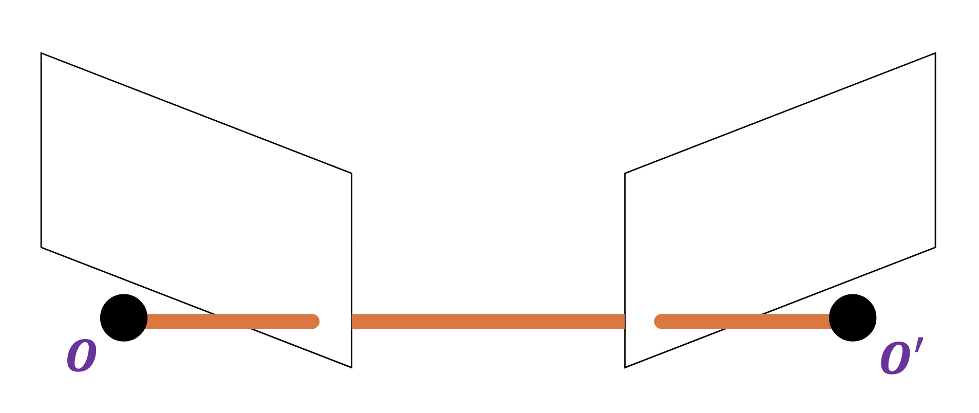
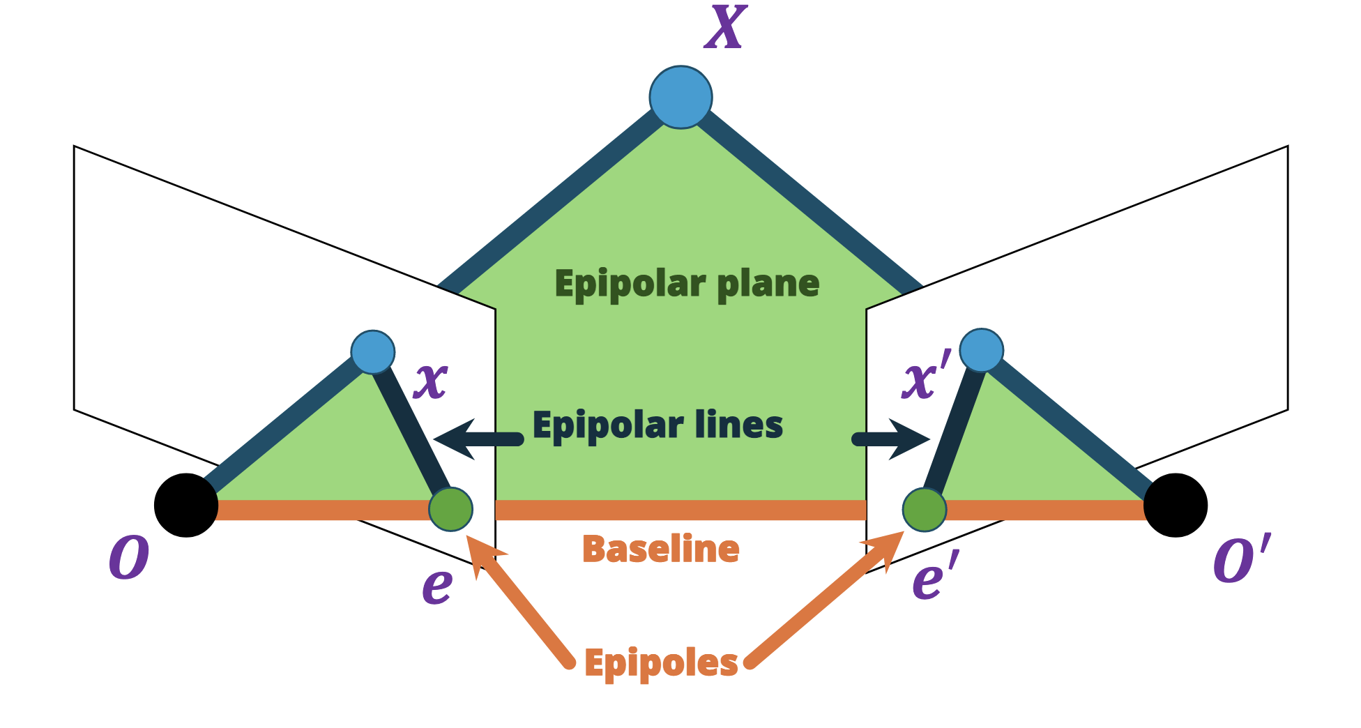
Suppose we have two cameras with centres $O$ and $O'$. @Define and @visualise the baseline.
The baseline is the line connecting the two origins.
Suppose we have two cameras with centres $O$ and $O'$ connected by their baseline.
@Define and @visualise the epipoles $e$ and $e$’. What does this look like when the cameras lie on the same line?
The epipoles are where the baseline intersects with the image plane (equivalently, the projections of the other camera in each view).
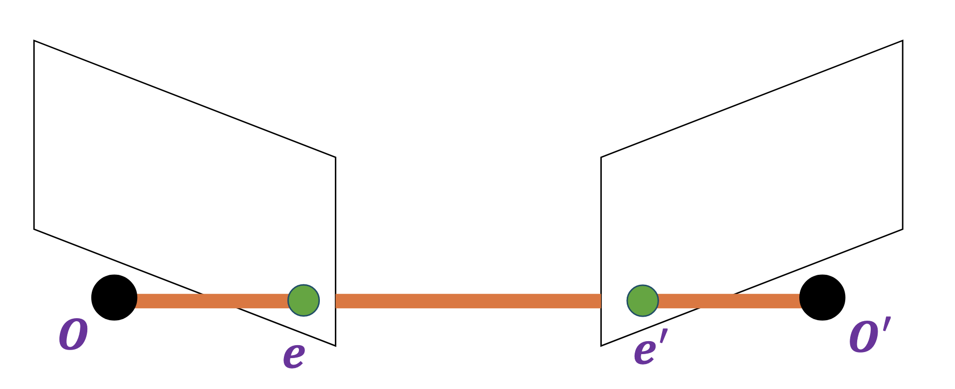
When the baseline is parallel to the image planes (the “motion parallel to image plane” case, e.g. a lateral stereo rig), the epipoles are infinitely far away and the epipolar lines are parallel.
Suppose we have two cameras with centres $O$ and $O'$ with epipoles $e$ and $e'$, along with a point $X$ which projects onto $x$ and $x'$ respectively.
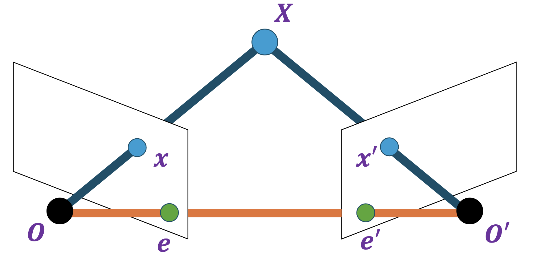
@Define and visualise the epipolar plane and the epipolar lines in this context.
- The epipolar plane is the plane formed by $X$, $O$ and $O'$.
- The epipolar lines connect the epipoles to the projections of $X$, or equivalently the intersection of the epipolar plane with the image plane.
Suppose we observe a single point $x$ in some image taken by a camera with centre $O$.
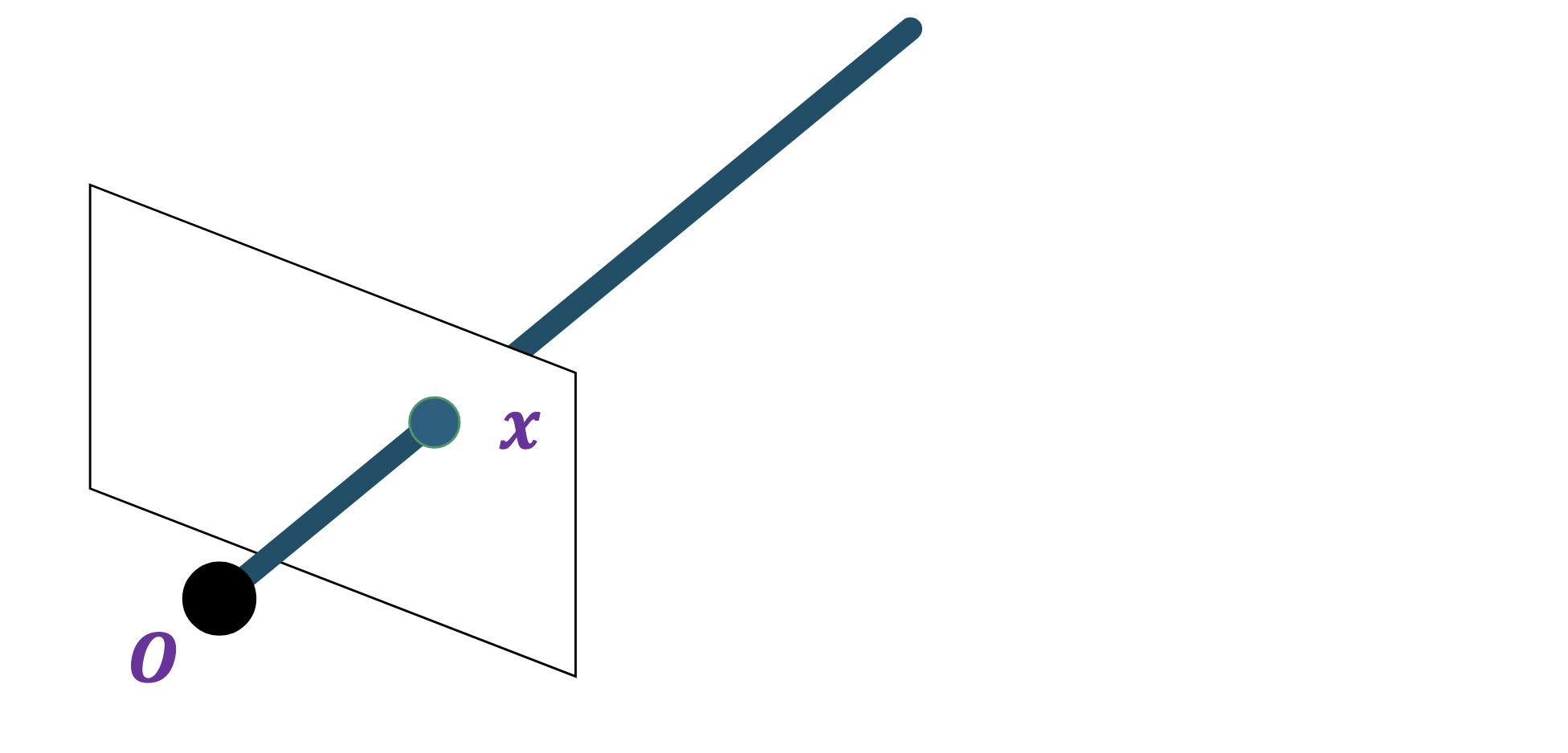
Given another camera with centre $O'$, where can we find the $x'$ corresponding to the $x$ in the other image?
Along the epipolar line corresponding to $x$.
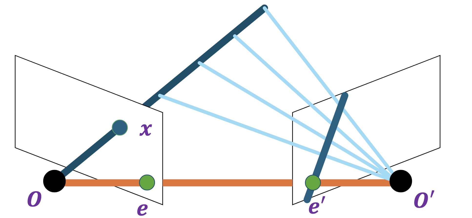
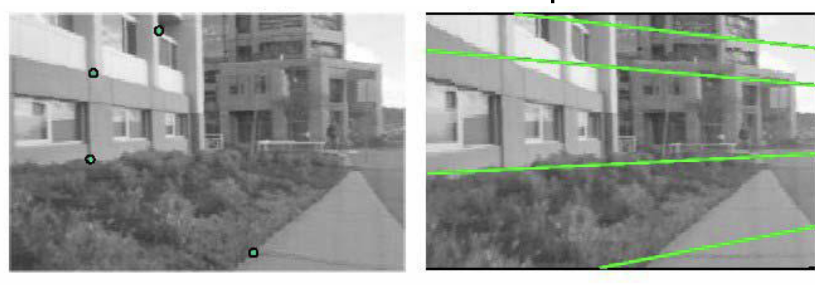
@Visualise what the epipolar lines would look like given a reference image and a target image.
@State and @visualise the epipolar constraint.
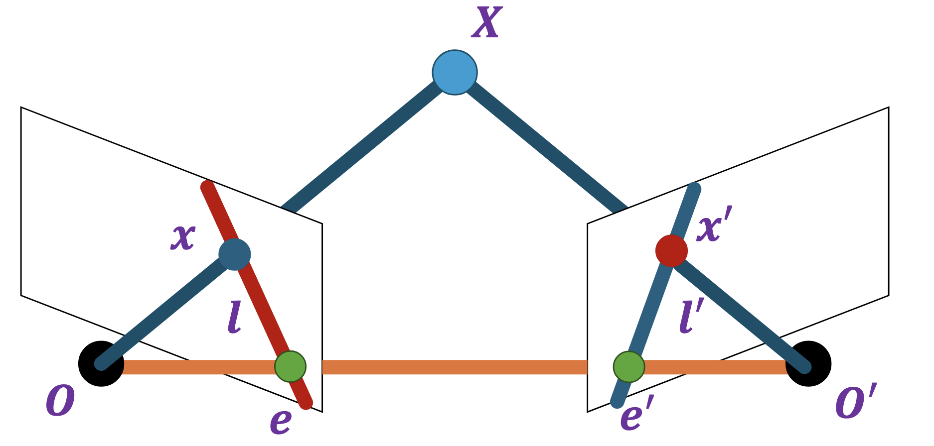
Whenever two points $x$ and $x'$ lie on matching epipolar lines $l$ and $l'$, the visual rays corresponding to them meet in space at some point $X$ (although they do not have to be projections of the same 3D point)
Consider the following setup:
- We have two cameras at points $O$ and $O'$, of which the intrinsic $K, K'$ and extrinsic parameters are known
- The world coordinate system is set to that of the first camera
- The rotation and translation from $O$ to $O'$ is given as above
What are the two projection matrices $P, P'$ from the world coordinates to the camera coordinates?
- $K[I \mid 0]$
- $K'[R \mid t]$
Consider the following setup:
- We have two cameras at points $O$ and $O'$, of which the intrinsic $K, K'$ and extrinsic parameters are known
- The world coordinate system is set to that of the first camera
- The rotation and translation from $O$ to $O'$ is given as above, so that the projection matrices are given by $K[I \mid 0]$ and $K'[R \mid t]$
Given $X$, $x _ \text{pixel}$ and $x' _ \text{pixel}$, where are $x$ and $x'$ in normalised image coordinates?
- $x _ \text{norm} = K^{-1} x _ \text{pixel} \cong [I \mid 0] X$
- $x' _ \text{norm} = {K'}^{-1} x' _ \text{pixel} \cong [R \mid t]X$
Consider the following setup:
- We have two cameras at points $O$ and $O'$, of which the intrinsic $K, K'$ and extrinsic parameters are known
- The world coordinate system is set to that of the first camera
- The rotation and translation from $O$ to $O'$ is given as above, so that the projection matrices are given by $K[I \mid 0]$ and $K'[R \mid t]$
- To simplify, we work in normalised image coordinates: given $X$, $x _ \text{pixel}$ and $x' _ \text{pixel}$, we have
- $x _ \text{norm} = K^{-1} x _ \text{pixel} \cong [I \mid 0] X$
- $x' _ \text{norm} = {K'}^{-1} x' _ \text{pixel} \cong [R \mid t]X$
@State four different ways of expressing the relationship between $x$ and $x'$:
- By simply stating their exact relationship
- Using the cross product
- Using the “matrix form” of the cross product
- Using the essential matrix
- $x _ \text{norm} = K^{-1} x _ \text{pixel} \cong [I \mid 0] X$
- $x' _ \text{norm} = {K'}^{-1} x' _ \text{pixel} \cong [R \mid t]X$
Stating their exact relationship:
The direct transformation between $x$ and $x'$ gives
\[x' \cong Rx + t\]This means that $x'$, $Rx$ and $t$ are linearly dependent, so:
Using the cross product:
\[x' \cdot [t \times (Rx)] = 0\]Since
\[a \times b = \begin{bmatrix} 0 & -a _ 3 & a _ 2 \\ a _ 3 & 0 & -a _ 1 \\ -a _ 2 & a _ 1 & 0 \end{bmatrix} \begin{pmatrix} b _ 1 \\ b _ 2 \\ b _ 3 \end{pmatrix} := [a _ \times] b\]we have:
Using the “matrix form” of the cross product:
\[x'^\top [t _ \times] Rx = 0\]so defining $[t _ x] R = E$ as the “essential matrix”:
Using the essential matrix:
\[x'^\top E x = 0\]Consider the following setup:
- We have two cameras at points $O$ and $O'$, of which the intrinsic $K, K'$ and extrinsic parameters are known
- The world coordinate system is set to that of the first camera
- The rotation and translation from $O$ to $O'$ is given as above, so that the projection matrices are given by $K[I \mid 0]$ and $K'[R \mid t]$
- To simplify, we work in normalised image coordinates: given $X$, $x _ \text{pixel}$ and $x' _ \text{pixel}$, we have
- $x _ \text{norm} = K^{-1} x _ \text{pixel} \cong [I \mid 0] X$
- $x' _ \text{norm} = {K'}^{-1} x' _ \text{pixel} \cong [R \mid t]X$
Then the direct transformation between $x$ and $x'$ gives
\[x' \cong Rx + t\]
this means that $x'$, $Rx$ and $t$ are linearly dependent, so we have
\[x' \cdot [t \times (Rx)] = 0\]
Collecting this into matrix form and defining $[t _ x] R = E$ as the “essential matrix”, we have
\[x'^\top E x = 0\]
@State how you may:
- Determine the epipolar line $l'$ corresponding to a point $x$
- Determine the epipolar line $l$ corresponding to a point $x'$
- $x _ \text{norm} = K^{-1} x _ \text{pixel} \cong [I \mid 0] X$
- $x' _ \text{norm} = {K'}^{-1} x' _ \text{pixel} \cong [R \mid t]X$
- $l' \cong Ex$
- $l \cong E^\top x'$
Consider the following setup:
- We have two cameras at points $O$ and $O'$, of which the intrinsic $K, K'$ and extrinsic parameters are known
- The world coordinate system is set to that of the first camera
- The rotation and translation from $O$ to $O'$ is given as above, so that the projection matrices are given by $K[I \mid 0]$ and $K'[R \mid t]$
- To simplify, we work in normalised image coordinates: given $X$, $x _ \text{pixel}$ and $x' _ \text{pixel}$, we have
- $x _ \text{norm} = K^{-1} x _ \text{pixel} \cong [I \mid 0] X$
- $x' _ \text{norm} = {K'}^{-1} x' _ \text{pixel} \cong [R \mid t]X$
Then the direct transformation between $x$ and $x'$ gives
\[x' \cong Rx + t\]
this means that $x'$, $Rx$ and $t$ are linearly dependent, so we have
\[x' \cdot [t \times (Rx)] = 0\]
Collecting this into matrix form and defining $[t _ x] R = E$ as the “essential matrix”, we have
\[x'^\top E x = 0\]
@State the relationship between the essential matrix $E$ and the epipolar points $e$ and $e'$.
- $x _ \text{norm} = K^{-1} x _ \text{pixel} \cong [I \mid 0] X$
- $x' _ \text{norm} = {K'}^{-1} x' _ \text{pixel} \cong [R \mid t]X$
- $Ee = 0$
- $E^\top e' = 0$
Consider the following setup:
- We have two cameras at points $O$ and $O'$, of which the intrinsic $K, K'$ and extrinsic parameters are known
- The world coordinate system is set to that of the first camera
- The rotation and translation from $O$ to $O'$ is given as above, so that the projection matrices are given by $K[I \mid 0]$ and $K'[R \mid t]$
- To simplify, we work in normalised image coordinates: given $X$, $x _ \text{pixel}$ and $x' _ \text{pixel}$, we have
- $x _ \text{norm} = K^{-1} x _ \text{pixel} \cong [I \mid 0] X$
- $x' _ \text{norm} = {K'}^{-1} x' _ \text{pixel} \cong [R \mid t]X$
Then the direct transformation between $x$ and $x'$ gives
\[x' \cong Rx + t\]
this means that $x'$, $Rx$ and $t$ are linearly dependent, so we have
\[x' \cdot [t \times (Rx)] = 0\]
Collecting this into matrix form and defining $[t _ x] R = E$ as the “essential matrix”, we have
\[x'^\top E x = 0\]
@State the rank and the degrees of freedom of $E$.
- $x _ \text{norm} = K^{-1} x _ \text{pixel} \cong [I \mid 0] X$
- $x' _ \text{norm} = {K'}^{-1} x' _ \text{pixel} \cong [R \mid t]X$
- Rank: $2$, so that $E$ is singular ($\det E = 0$)
- Why? $R$ is a rotation matrix, hence invertible, so $\text{rank}(E) = \text{rank}([t] _ \times)$. The cross-product matrix $[t] _ \times$ sends $v \mapsto t \times v$, so $t \times t = 0$, the vector $t$ lies in its null space. So $[t] _ \times$ has rank at most $2$, and exactly $2$ for any non-zero $t$.
- Degrees of freedom: $5$.
- Why? $R$ contributes 3 degrees of freedom (a rotation has three parameters), and $t$ contributes 3 degrees of freedom. The epipolar constraint $x'^\top E x = 0$ is invariant to scaling $E$ by any scalar, so $E$ is only defined up to scale, removing 1 degree of freedom.
Consider the following setup:
- We have two cameras at points $O$ and $O'$, of which the intrinsic $K, K'$ and extrinsic parameters are known
- The world coordinate system is set to that of the first camera
- The rotation and translation from $O$ to $O'$ is given as above, so that the projection matrices are given by $K[I \mid 0]$ and $K'[R \mid t]$
- To simplify, we work in normalised image coordinates: given $X$, $x _ \text{pixel}$ and $x' _ \text{pixel}$, we have
- $x _ \text{norm} = K^{-1} x _ \text{pixel} \cong [I \mid 0] X$
- $x' _ \text{norm} = {K'}^{-1} x' _ \text{pixel} \cong [R \mid t]X$
Then the direct transformation between $x$ and $x'$ gives
\[x' \cong Rx + t\]
this means that $x'$, $Rx$ and $t$ are linearly dependent, so we have
\[x' \cdot [t \times (Rx)] = 0\]
Collecting this into matrix form and defining $[t _ x] R = E$ as the “essential matrix”, we have
\[x'^\top E x = 0\]
What assumptions do we drop in order to @define the fundamental matrix?
- $x _ \text{norm} = K^{-1} x _ \text{pixel} \cong [I \mid 0] X$
- $x' _ \text{norm} = {K'}^{-1} x' _ \text{pixel} \cong [R \mid t]X$
- We assume that the calibration matrices $K$ and $K'$ of the two cameras are unknown
- This gives $x'^\top F x = 0$ where $F = (K'^{-1})^\top E K^{-1}$
Consider the following setup:
- We have two cameras at points $O$ and $O'$, of which the intrinsic $K, K'$ and extrinsic parameters are known
- The world coordinate system is set to that of the first camera
- The rotation and translation from $O$ to $O'$ is given as above, so that the projection matrices are given by $K[I \mid 0]$ and $K'[R \mid t]$
- To simplify, we work in normalised image coordinates: given $X$, $x _ \text{pixel}$ and $x' _ \text{pixel}$, we have
- $x _ \text{norm} = K^{-1} x _ \text{pixel} \cong [I \mid 0] X$
- $x' _ \text{norm} = {K'}^{-1} x' _ \text{pixel} \cong [R \mid t]X$
Then the direct transformation between $x$ and $x'$ gives
\[x' \cong Rx + t\]
this means that $x'$, $Rx$ and $t$ are linearly dependent, so we have
\[x' \cdot [t \times (Rx)] = 0\]
Collecting this into matrix form and defining $[t _ x] R = E$ as the “essential matrix”, we have
\[x'^\top E x = 0\]
For the fundamental matrix, we drop some assumptions:
- We assume that the calibration matrices $K$ and $K'$ of the two cameras are unknown
- This gives $x'^\top F x = 0$ where $F = (K'^{-1})^\top E K^{-1}$
@State:
- How you would determine the epipolar line $l'$ corresponding to a point $x$
- How you would determine the epipolar line $l$ corresponding to a point $x'$
- The relationship between the fundamental matrix $F$ and the epipolar points $e$ and $e'$.
- $x _ \text{norm} = K^{-1} x _ \text{pixel} \cong [I \mid 0] X$
- $x' _ \text{norm} = {K'}^{-1} x' _ \text{pixel} \cong [R \mid t]X$
- $l' \cong Fx$
- $l \cong F^\top x'$
- $Fe = 0$
- $F^\top e' = 0$
Consider the following setup:
- We have two cameras at points $O$ and $O'$, of which the intrinsic $K, K'$ and extrinsic parameters are known
- The world coordinate system is set to that of the first camera
- The rotation and translation from $O$ to $O'$ is given as above, so that the projection matrices are given by $K[I \mid 0]$ and $K'[R \mid t]$
- To simplify, we work in normalised image coordinates: given $X$, $x _ \text{pixel}$ and $x' _ \text{pixel}$, we have
- $x _ \text{norm} = K^{-1} x _ \text{pixel} \cong [I \mid 0] X$
- $x' _ \text{norm} = {K'}^{-1} x' _ \text{pixel} \cong [R \mid t]X$
Then the direct transformation between $x$ and $x'$ gives
\[x' \cong Rx + t\]
this means that $x'$, $Rx$ and $t$ are linearly dependent, so we have
\[x' \cdot [t \times (Rx)] = 0\]
Collecting this into matrix form and defining $[t _ x] R = E$ as the “essential matrix”, we have
\[x'^\top E x = 0\]
For the fundamental matrix, we drop some assumptions:
- We assume that the calibration matrices $K$ and $K'$ of the two cameras are unknown
- This gives $x'^\top F x = 0$ where $F = (K'^{-1})^\top E K^{-1}$
@State the rank and degrees of freedom of $F$.
- $x _ \text{norm} = K^{-1} x _ \text{pixel} \cong [I \mid 0] X$
- $x' _ \text{norm} = {K'}^{-1} x' _ \text{pixel} \cong [R \mid t]X$
- Rank: $2$, so $F$ is singular ($\det F = 0$).
- Why? $K$, $L'$ are upper triangular with non-zero diagonal entries (focal length, pixel scaling factors), so they’re invertible. Multiplying by invertible matrices preserves rank, so $\text{rank}(F) = \text{rank}(E) = 2$.
- Degrees of freedom: $7$.
- Why? A $3 \times 3$ matrix has $9$ entries. Subtract $1$ for scale (since $x'^\top F x = 0$ is invariant to scaling $F$). Subtract another $1$ for the rank-2 constraint $\det F = 0$. Hence we have rank $9 - 1 - 1 = 7$.
- Why more than $E$? $F$ absorbs the unknown calibration matrices.
Given that the fundamental matrix satisfies the equation
\[x'^\top F x = 0\]
Derive the eight-point algorithm for determining an estimate of $F$.
Explicitly, we require for each pair of points $\pmb x, \pmb x'$
\[\begin{bmatrix} x' \\ y' \\ 1 \end{bmatrix}^\top \begin{bmatrix} f _ {11} & f _ {12} & f _ {13} \\ f _ {21} & f _ {22} & f _ {23} \\ f _ {31} & f _ {32} & f _ {33} \end{bmatrix} \begin{bmatrix} x \\ y \\ 1 \end{bmatrix} = 0\]which, vectorising $f$ gives
\[\begin{pmatrix} x'x & x'y & x' &y'x & y'y & y' & x & y & 1 \end{pmatrix} \begin{pmatrix} f _ {11} \\ f _ {12} \\ f _ {13} \\ f _ {21} \\ f _ {22} \\ f _ {23} \\ f _ {31} \\ f _ {32} \\ f _ {33} \\ \end{pmatrix} = 0\]Collecting this into a matrix equation for each of the point correspondences, we have
\[Uf = 0\]where
\[\begin{aligned} U &= \begin{pmatrix} x _ 1'x _ 1 & x _ 1'y _ 1 & x _ 1' & y _ 1'x _ 1 & y _ 1'y _ 1 & y _ 1' & x _ 1 & y _ 1 & 1 \\ & & & & \vdots & & & & \\ x _ n'x _ n & x _ n'y _ n & x _ n' & y _ n'x _ n & y _ n'y _ n & y _ n' & x _ n & y _ n & 1 \\ \end{pmatrix} \\ \\ \end{aligned}\]which can be solved via least squares. To enforce the fact $F$ must be rank $2$, we can take the best rank-2 approximation of the found solution using truncated SVD.
@State the geometric meaning of the epipolar constraint $\pmb x'^\top E \pmb x = 0$, and explain why this picture is the foundation of multi-view geometry.
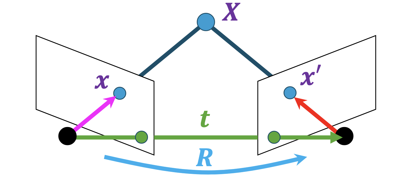
The geometric picture: a 3D point $\pmb X$ together with the two camera centres $O, O'$ defines a plane in space, the epipolar plane. The two image points $\pmb x, \pmb x'$ are by construction the projections of $\pmb X$ along the rays from $O$ and $O'$, so they also lie in this plane. Thus all five points $\{\pmb X, O, O', \pmb x, \pmb x'\}$ are coplanar. The epipolar constraint is the algebraic encoding of this single fact.
Encoding into algebra: in camera 2’s frame, the three vectors $\pmb x'$, $R\pmb x$, and $\pmb t$ (all radiating from $O'$, where $\pmb t$ is the position of $O$ in camera 2’s frame) are coplanar iff their scalar triple product vanishes: $\pmb x' \cdot (\pmb t \times R\pmb x) = 0$. Rewriting the cross product as a matrix multiplication (∆cross-product) and absorbing $[\pmb t] _ \times R$ into the essential matrix $E$ gives $\pmb x'^\top E \pmb x = 0$. The fuller algebraic derivation is in ∆essential-matrix-four-derivations.
Why this picture is the foundation of MVG:
- It is the reason matching reduces from a 2D to a 1D search: given $\pmb x$ in the first image, the matching $\pmb x'$ must lie in the epipolar plane, hence in the epipolar plane’s projection into image 2, which is exactly the epipolar line $\ell' = E\pmb x$.
- It is necessary but not sufficient for $\pmb x, \pmb x'$ to be true correspondences (∆bite-epipolar-constraint-necessary-not-sufficient): two arbitrary points on matching epipolar lines also satisfy the constraint without being projections of the same 3D point.
- It is the geometric reason for the rank-2 property of $E$ and $F$ (∆bite-essential-matrix-rank2-justification): every epipolar line passes through the epipole, so $E$ has a non-trivial null space.
- Stereo rectification, triangulation, structure-from-motion, and bundle adjustment all build on this single picture.
@State the relationship between two views of a planar scene, justify it geometrically, and contrast it with the relationship for a general scene.
If all observed 3D points lie on a single plane $\Pi$, then for every pair of matching image points there is a $3 \times 3$ homography $H$ with $\pmb x' \cong H \pmb x$.
Why: a plane $\Pi$ is itself a 2D space. View 1’s projection restricted to $\Pi$ is a bijection between $\Pi$ and image 1, and similarly for view 2. Composing image-1 $\to \Pi \to$ image-2 gives a 2D-to-2D map that is linear in homogeneous coordinates, hence a homography.
Contrast with the general (non-planar) case: a general scene gives only the epipolar constraint $\pmb x'^\top F \pmb x = 0$, which pins $\pmb x'$ to a line (1 equation per point). The planar case pins $\pmb x'$ to a point $H\pmb x$ (2 equations per point), strictly stronger because the planar assumption removes one DoF.
Practical implications:
- Planar scenes need only 4 correspondences to determine the relationship (∆homography-min-correspondences), versus 8 for $F$ (∆bite-eight-point-minimum-correspondences).
- This is the implicit assumption behind SIFT’s geometric verification (∆sift-planar-assumption).
- A pure-rotation camera (about a fixed centre) is equivalent to viewing the plane at infinity, so panorama stitching is also a homography problem.
@State the four main uses of the fundamental matrix $F$ (and the essential matrix $E$) in two-view geometry, and explain why they are the central objects of MVG.
The fundamental and essential matrices are the central objects of two-view geometry because they encode the geometric relationship between two views in a single $3 \times 3$ matrix. The slogan: $F$ is “the geometry between two views”, and almost anything you want to do with two views flows from it.
Use 1, matching, reduce a 2D search to 1D. Naive correspondence search between two images is $O(N^2)$ in the number of pixels. The epipolar constraint $\pmb x'^\top F \pmb x = 0$ pins the matching $\pmb x'$ to the line $F\pmb x$ in image 2 (∆epipolar-coplanarity), so matching reduces to a 1D scan along that line. This is what makes stereo matching tractable.
Use 2, calibration-free reconstruction. $F$ can be estimated from 2D-2D correspondences alone (∆eight-point-algorithm-derivation), with no knowledge of intrinsics. This is what enables reconstruction from random internet photos taken on unknown cameras (Photo Tourism, COLMAP).
Use 3, relative camera motion. $E = [\pmb t] _ \times R$, so once $E$ is estimated (8-point on normalised coordinates, or 5-point directly), an SVD decomposition recovers the relative rotation $R$ and translation $\pmb t$ up to a 4-fold ambiguity (resolved by cheirality, i.e. requiring reconstructed points to lie in front of both cameras).
Use 4, inlier filtering for noisy matches. Real correspondences (from SIFT etc.) are noisy. Fitting $F$ via RANSAC gives a geometric model that separates true matches from spurious ones. This is what makes SfM robust in practice.
Without $F$ or $E$: no efficient matching, no relative pose recovery, no triangulation, no SfM. Every pipeline in classical multi-view reconstruction routes through this single $3 \times 3$ object.
You have already estimated the fundamental matrix $F$ relating two views (or, for calibrated cameras in normalised coordinates, the essential matrix $E = [\pmb t] _ \times R$). True correspondences satisfy $\pmb x'^\top F \pmb x = 0$, and the epipolar line of $\pmb x$ in the second image is $\ell' = F\pmb x$.
@Describe how $F$ (or $E$) is then used to determine correspondences, covering both finding a new match and verifying a candidate one.
The headline: the match for $\pmb x$ must lie on its epipolar line $\ell' = F\pmb x$ (∆matching-point-on-epipolar-line), so $F$ turns 2D matching into a 1D search. This is necessary, not sufficient (∆bite-epipolar-constraint-necessary-not-sufficient): it pins $\pmb x'$ to a line, it does not pick the point on it.
Guided matching (find a new match):
- Compute the epipolar line $\ell' = F\pmb x$ (∆fundamental-matrix-epipolar-lines-and-epipoles).
- Search only along $\ell'$ (a 1D scan, not the whole image), scoring a patch / descriptor around $\pmb x$ against candidates on the line and taking the lowest-cost one.
Verification (filter a candidate pair $(\pmb x, \pmb x')$):
- Accept iff $\pmb x'$ lies close to its epipolar line, $d(\pmb x', F\pmb x) < \tau$ (point-to-line distance, equivalently a normalised $ \vert \pmb x'^\top F \pmb x \vert $).
- This is exactly the RANSAC inlier test that both estimates $F$ and strips out false SIFT matches (∆bite-geometric-verification-ransac).
Dense version (stereo): rectify the pair so epipolar lines become corresponding horizontal scanlines (the motion-parallel-to-image-plane case, ∆bite-epipolar-geometry-three-cases); each pixel’s match is then on the same row, and the offset along it (the disparity) gives depth.
Bootstrap: you need matches to estimate $F$ in the first place (eight-point + RANSAC, ∆eight-point-algorithm-derivation), so the loop is sparse SIFT matches → RANSAC-fit $F$ → use $F$ to verify and to densify by epipolar search.
Bite-sized
The essential matrix $E = [t] _ \times R$ was introduced by Longuet-Higgins, Nature 1981 in the paper “A computer algorithm for reconstructing a scene from two projections”. The eight-point algorithm for estimating $F$ from correspondences was popularised by Hartley in 1997.
The eight-point algorithm requires at minimum 8 point correspondences to estimate the fundamental matrix $F$ (which has 9 entries, defined up to scale, giving 8 unknowns). With more than 8 correspondences, solve via least squares.
@Describe how rank-2 enforcement via SVD truncation works in the eight-point algorithm, and why it’s necessary.
The eight-point algorithm gives an initial estimate $F _ \text{init}$ from a least-squares fit to $Uf = 0$. Because the constraint $\det F = 0$ is not directly enforced during the least-squares solve, $F _ \text{init}$ is typically full rank — but the true fundamental matrix must be rank 2.
Why rank-2 is required: $F$ has the geometric meaning that $Fx$ is the epipolar line of $x$; all epipolar lines must pass through the epipole $e'$, which means $F^\top e' = 0$, so $F$ must have a non-trivial null space, i.e. rank $< 3$. A full-rank $F _ \text{init}$ would predict epipolar lines that don’t quite converge at the epipole — physically impossible.
The fix: take the SVD of the initial estimate
\[F _ \text{init} = U \Sigma V^\top, \quad \Sigma = \mathrm{diag}(\sigma _ 1, \sigma _ 2, \sigma _ 3),\]zero out the smallest singular value,
\[\Sigma' = \mathrm{diag}(\sigma _ 1, \sigma _ 2, 0),\]and reconstruct
\[F = U \Sigma' V^\top.\]This gives the closest rank-2 matrix to $F _ \text{init}$ in Frobenius norm (Eckart-Young theorem), and produces an $F$ whose epipolar lines actually meet at a single epipole.
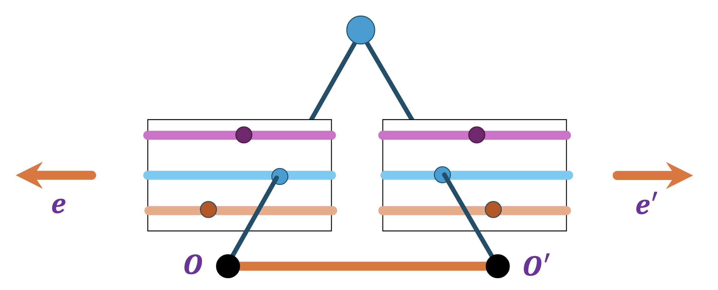
@Describe the three special configurations of epipolar geometry covered in the lecture.
- Converging cameras (general case): the baseline lies in front of both image planes, so the epipoles are finite points and may even be visible inside one of the images. Epipolar lines fan out from the visible epipole. Standard case.
- Motion parallel to the image plane (e.g. a lateral stereo rig with both cameras facing forward): the baseline is parallel to both image planes, so the epipoles are at infinity, and the epipolar lines are parallel horizontal lines in both images. Stereo-rectified images are normalised to this case.
- Motion perpendicular to the image plane (e.g. a camera moving directly forward): the epipoles coincide with the principal points of both cameras, and epipolar lines radiate outward from the principal point (the focus of expansion). Useful for monocular depth estimation from forward motion.
@Justify why the epipolar constraint $\pmb x'^\top E \pmb x = 0$ is necessary but not sufficient for two image points to be projections of the same 3D point.
Necessary: If $\pmb x, \pmb x'$ are projections of the same 3D point $X$, then by construction $X, O, O'$ are coplanar (they define the epipolar plane), which translates algebraically to the epipolar constraint $\pmb x'^\top E \pmb x = 0$. So genuine correspondences always satisfy the constraint.
Not sufficient: The constraint only says $\pmb x'$ lies on the epipolar line $\ell' = E \pmb x$ — a 1D locus in the second image. There are many 3D points whose rays from the second camera all lie in the same epipolar plane and so project to different points on $\ell'$. Picking any of them gives a different $\pmb x'$ that still satisfies the constraint but corresponds to a different 3D point.
Geometrically: the epipolar constraint reduces a 2D search (the whole second image) to a 1D search (the epipolar line), but you still need a matching step (intensity, descriptor, or local cost) to find the actual corresponding point on $\ell'$.
@Justify the rank-2 property of the essential matrix $E = [t] _ \times R$.
The cross-product matrix $[t] _ \times$ has rank at most 2 for any non-zero $t$: it sends $\pmb v \mapsto t \times \pmb v$, and $t \times t = \pmb 0$, so $t$ is always in its null space — making its kernel at least 1-dimensional. For a 3D vector $t \ne 0$, the kernel is exactly 1-dimensional, so $\mathrm{rank}([t] _ \times) = 2$.
$R$ is a rotation matrix, hence orthogonal and invertible (rank 3). Multiplying $[t] _ \times$ on the right by an invertible matrix doesn’t change the rank:
\[\mathrm{rank}(E) = \mathrm{rank}([t] _ \times R) = \mathrm{rank}([t] _ \times) = 2.\]Equivalently: $E^\top e' = 0$ for the epipole $e'$, so $E^\top$ has a non-trivial null space.
The relationship $F = (K')^{-\top} E K^{-1}$ shows that the fundamental matrix is essentially the essential matrix expressed in pixel rather than normalised coordinates. Since $K, K'$ are invertible (upper triangular with positive diagonal), $F$ has the same rank as $E$ (namely 2), but $F$ has 7 DoF rather than 5 because it also absorbs the unknown calibration.
Visualising epipolar geometry
The whole of two-view geometry is easier to see in 3D. Orbit the scene and move the point X and the second camera. The epipolar plane through O, O’ and X is drawn explicitly, so the ∆essential-matrix-four-derivations coplanarity of $x'$, $Rx$ and $t$ becomes literal: the three vectors all lie in that plane, and $x'^\top E x = 0$ is just that triple product vanishing. The image panels show the ∆epipolar-plane-and-lines, so the line $l' = Ex$ in camera 2 is the search line on which the match $x'$ must lie, and the explainer notes how the ∆fundamental-matrix-from-uncalibrated $F = (K')^{-\top} E K^{-1}$ is the same object in pixel rather than normalised coordinates. The other tabs reuse the scene for triangulation (two rays meeting at X, and how noise makes them miss) and for homographies (a plane, or a pure rotation, mapping one image to the other by a single $3\times 3$ matrix).