Computer Vision MT25, Sampling and reconstruction


Flashcards

@Define sampling.

Recording the values of a function at a discrete set of locations.

@Define reconstruction.

Converting a sampled representation of a function back into a continuous function by “guessing” what happens between the samples.

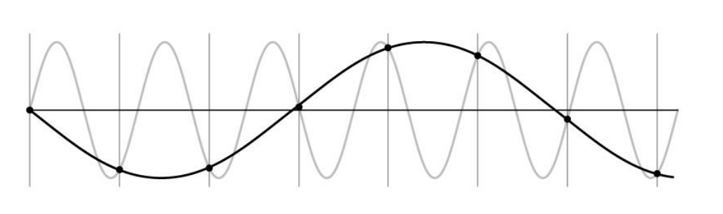
@Visualise why it’s important that you sample a signal with a sufficiently high frequency.
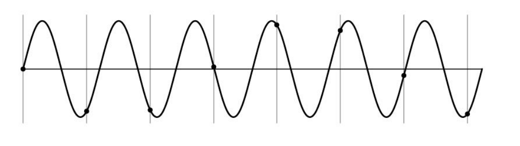
Here is a signal for you to consider:

@Define aliasing.

The distortion of high-frequency content in a signal when it is sampled at an insufficient rate.

@State the Nyquist-Shannon sampling theorem.

When sampling a signal at discrete intervals, the sampling frequency must be at least twice the maximum frequency of the input signal to allow perfect reconstruction of the original signal.

@Describe two ways that you could prevent aliasing.

  • Sample more often
  • Remove all frequencies greater than half the sampling frequency, e.g. using smoothing or a low-pass filter

Bite-sized

The Nyquist-Shannon sampling theorem says the sampling frequency must be at least twice the maximum frequency in the signal for perfect reconstruction. Equivalently, the sampling period must be at most $1/(2 f _ \text{max})$ — half the period of the fastest content.

Source: Lecture 2, Nyquist-Shannon Sampling Theorem slide.

@bite~

@Describe three real-world examples of aliasing artefacts in images.

  • Disintegrating textures: a regular pattern (e.g. a red-and-white checkerboard) viewed in perspective appears to “break down” into noise where the pattern’s spatial frequency exceeds the local pixel resolution. The fine far-away squares cannot be resolved by individual pixels, so the sampled image looks like random noise rather than a regular pattern.
  • Moiré patterns: photographing a fine repetitive pattern (fabric, screen door, fence) produces a visible secondary pattern at a much lower frequency than the original. The camera’s pixel grid and the pattern’s spatial frequency beat against each other.
  • False colour: a zoomed-in view of a screen shows coloured fringing around edges. The Bayer-pattern colour sensor cannot resolve the subpixel content, so it reconstructs colours that aren’t there.

All three are the same phenomenon — high-frequency signal masquerading as low-frequency content because the sampling rate is too low.

Source: Lecture 2, Aliasing “in the Wild” slide.

@bite~

@Justify the anti-aliasing procedure of blur-before-downsample in terms of frequency content.

Naive subsampling (just throw away every other pixel) reduces the effective sampling rate. If the original signal has frequency content above the new Nyquist limit, aliasing produces visible noise in high-frequency regions.

The fix is to low-pass filter the signal before subsampling, removing all frequencies above the new Nyquist limit. Then there’s no high-frequency content to alias.

Why Gaussian blur is the standard anti-alias filter:

  • Smoothly attenuates high frequencies without sharp cutoff (which would cause ringing).
  • Frequency-domain Gaussian (the FT of a Gaussian) has no sidelobes, unlike a box filter (whose FT is a sinc with prominent sidelobes).
  • Separable and cheap to compute.

You’re trading high-frequency content (which would alias) for slightly blurry output. This is always worth it: any high-frequency content that would have aliased was already corrupted in the sampled image.

Source: Lecture 2, Subsampling with Anti-aliasing slide.

@bite~

Aliasing is when sampled content “masquerades as” lower (or higher) frequency content — high-frequency signal that the sampler cannot resolve appears at an unrelated frequency in the sampled output. The lecture quote: signal traveling in disguise as other frequencies.

Source: Lecture 2, Aliasing in Sampling slide.

@bite~

Interpolation converts a sampled (discrete) image back into a continuous function for resampling at non-integer locations. The standard methods in order of smoothness: nearest-neighbour (piecewise constant), bilinear (piecewise linear in 2D), bicubic (smooth differentiable cubic spline).

Source: Lecture 2, Other Interpolation Schemes slide.

@bite~