Computer Vision MT25, Segmentation
Flashcards
In what way is image classification, object detection and segmentation all really the same task?
They are all instances of spatial labelling, at different levels of granularity:
- Image classification: Image-scale
- Object detection: Region-scale
- Segmentation: Pixel-scale
@Define semantic segmentation.
The task of labelling each pixel in an image with a category label, not differentiating instances.
What’s one way you could evaluate a segmentation model?
Do a per-class IoU of the predictions versus the ground truth.
How could you do segmentation with a sliding window approach?
Slide a window over the whole image and classify the centre pixel of the window.
What are the main drawbacks of sliding window segmentation?
- It is very inefficient: we are recomputing the same features for overlapping patches
- It is very noisy: separate predictions for each class
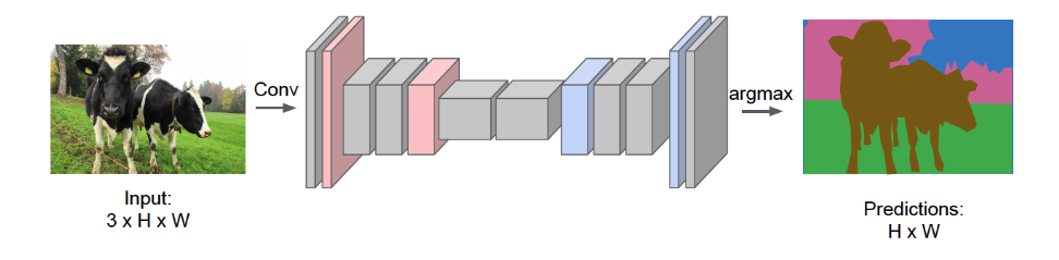
@Define and @visualise a fully convolutional network (FCN).
A CNN where you replace the final fully connected layers by convolutions and maintain the same input / output image size.
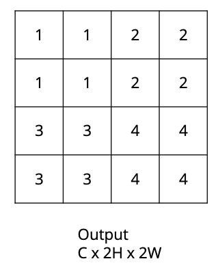
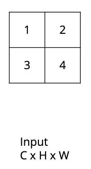
How would the nearest neighbour upsampling algorithm convert this $C \times H \times W$ image into a $C \times 2H \times 2W$ image?
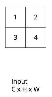
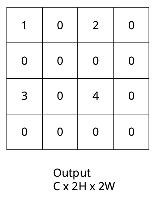
How would the bed of nails upsampling algorithm convert this $C \times H \times W$ image into a $C \times 2H \times 2W$ image?

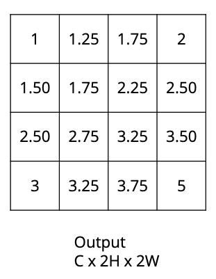
How would the bilinear interpolation upsampling algorithm convert this $C \times H \times W$ image into a $C \times 2H \times 2W$ image?

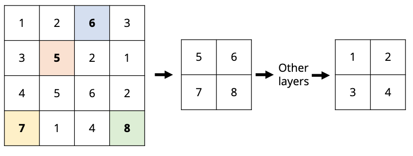
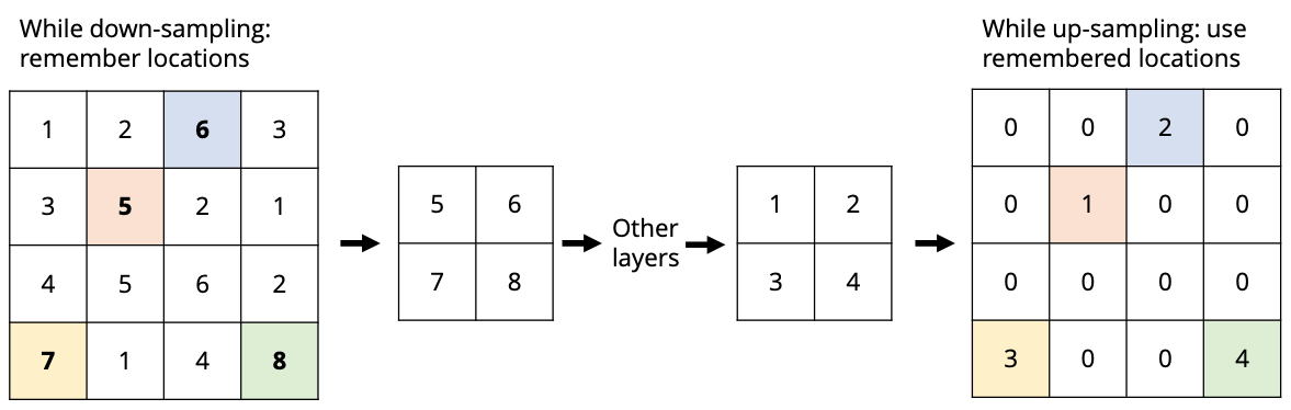
How would the max-unpooling upsampling algorithm convert this $C \times H \times W$ image into a $C \times 2H \times 2W$ image
given that this was down-sampled via
?
How would a transposed convolution (width, height 3 and stride 2) applied to the input square $a _ 1, a _ 2, a _ 3, a _ 4$ calculate the upsampled version?
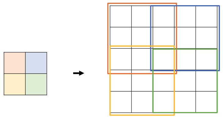
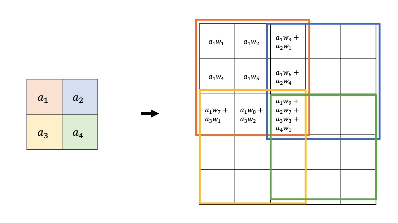

What artefacts do you typically get using transposed convolutions and how are these handled?
The repeated sums in the intersection points mean you get a grid-like pattern, you can fix this with another normal convolution.
What is the advantage of transposed convolutions compared to other upsampling techniques?

There are learnable weights.
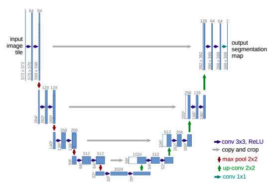
@Visualise a U-net and @describe two of its special features that made it particularly effective.
- Symmetric encoder-decoder structure: a contracting path of convolutions and pooling that produces low-resolution, high-semantic features, followed by an expanding path of upsampling that mirrors the contracting path.
- Skip connections via concatenation (not residual addition): each upsampled feature map in the decoder is concatenated channel-wise with the matching higher-resolution, lower-level feature map from the encoder. This brings local detail (edges, fine structure) back into the decoder, which the upsampled high-level features have lost.

@Describe the technique that the Segment Anything Model (SAM) used in order to gather such a large amount of supervised training data.
- Training with humans in the loop:
- Annotate data
- Train model
- Label more data with the model
- Humans fix and improve the labels
- Goto 2
@Define stuff.
Material defined by a homogeneous or repetitive pattern of fine-scale properties, but has no specific or distinctive spatial extent or shape.
@Define instance segmentation.
Detecting all objects (things) in an image, and identify the pixels that belong to each object.
@Visualise the difference between semantic segmentation and instance segmentation.
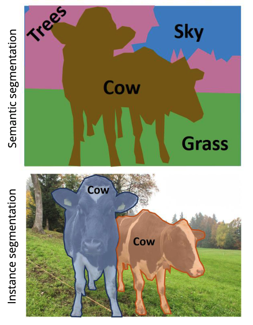
In instance segmentation, we want to detect all objects in an image and identify the pixels that belong to each object.
What might the intuitive approach be here, and what typically happens in practice?
- Intuitive approach:
- Detect objects
- Predict a segmentation mask for each object
- In practice:
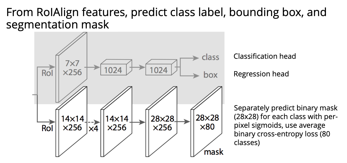
- Add another branch to an existing classification / bounding box regression model that outputs a segmentation mask for that region
How does RoIAlign improve over RoIPool?
RoIPool uses nearest neighbour quantisation to fill the fixed dimensional representation, RoIAlign instead uses bilinear interpolation of the feature map.
@Define the problem of panoptic segmentation.
Combine semantic segmentation for stuff with instance segmentation of things.
How does the keypoint problem differ from instance segmentation.
Instead of predicting a mask, you instead predict an object-specific landmark such as joints.
@Visualise what the keypoint masks for human pose estimation might look like, and @describe how this links to instance segmentation.
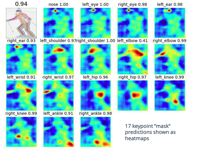
In instance segmentation, we would just predict a mask for the object. Here we predict a heatmap instead, and then convert the heatmap into a keypoint using e.g. a weighted sum over heatmap locations.
Suppose we have some heatmap $h$ corresponding to where we think a particular location in an object is:

How can you convert this heatmap into a single point $(p _ x, p _ y)^\top$?
Calculate
\[(p _ x, p _ y)^\top = \sum _ {u, v} \begin{pmatrix}u \\ v\end{pmatrix} H(u, v)\]where $H = \text{softmax}(h)$.
@Visualise the problem of dense captioning. @Describe how you might implement this.
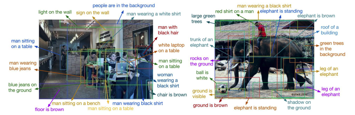
You could add another branch to the model with text output for each region.
@Describe the MaskFormer architecture for semantic segmentation.
Three modules built on a CNN / transformer backbone.
- Pixel-level module: the backbone produces image features $\mathcal F$, which a pixel decoder upsamples into per-pixel embeddings $\mathcal E _ \text{pixel} \in \mathbb R^{C _ \epsilon \times H \times W}$
- Transformer module: a transformer decoder takes $N$ learned queries and outputs:
- $N$ class predictions in $\mathbb R^{N \times (K+1)}$ via an MLP. The $+1$ is the “no object class”, trained with classification loss.
- $N$ mask embeddings $\mathcal E _ \text{mask} \in \mathbb R^{C _ \epsilon, N}$.
- Segmentation model:
- Each mask embedding is dotted with the per-pixel embeddings to give $N$ binary mask predictions in $\mathbb R^{N \times H \times W}$, trained with binary mask loss.
At inference, predictions assigned with “no object” are dropped and the remaining masks combine into a $K \times H \times W$ semantic segmentation.
Learned queries: the $N$ queries $Q \in \mathbb R^{N \times d}$ are model parameters, initialised randomly and trained by backprop alongside the rest of the network, not derived from any input sequence (unlike e.g. ViT where queries come from input patches, or translation transformers where they come from the target sequence). This is what decouples the output size from the input: the model always emits a fixed $N$ predictions regardless of how many objects are in the image, with unused slots assigned “no object” at inference. Each query gradually specialises during training (emergently, not hand-coded) via the Hungarian matching loss which is permutation-invariant across the $N$ slots.

@Describe the architecture of the Segment Anything Model (SAM).
Three modules:
- Image encoder: a heavy ViT (∆vision-transformer-architecture) encoder, run one per image, producing an image embedding.
- Prompt encoder: a lightweight encoder for the user prompt.
- Mask decoder: a lightweight transformer decoder that combines the image embedding with the prompt embedding into a binary segmentation mask.

Bite-sized
SAM (Segment Anything Model) was introduced by Kirillov et al., 2023 and trained on a dataset of $\sim 1$ billion masks across $\sim 11$ million images (SA-1B), built with humans-in-the-loop annotation. Its key innovation is the promptable interface: a user can supply seed points, scribbles, a bounding box, or even text to specify what to segment.
MaskFormer (Cheng, Schwing, Kirillov, NeurIPS 2021) reframes semantic segmentation as a mask classification task rather than per-pixel classification, by using $N$ learned object queries to predict $N$ candidate masks plus a class label per mask. This unification lets the same model do semantic, instance, and panoptic segmentation.
@Justify why concatenation (rather than residual addition) is used for U-Net’s skip connections.
U-Net’s encoder produces feature maps at multiple resolutions. The decoder upsamples its features and combines them with the encoder’s same-resolution maps via skip connections.
The choice:
- Residual addition $y = f(x) + x$ requires the encoder and decoder features to be in the same vector space — same number of channels with directly comparable semantics. After several layers of encoder-decoder processing, this assumption is dubious.
- Concatenation along the channel axis simply stacks the encoder and decoder features. The next conv layer then learns how to combine them, with no implicit assumption that they live in the same space.
For U-Net specifically, the encoder side has low-level features (edges, textures) and the decoder side has high-level features (semantics from the bottleneck). Concatenation lets the decoder use both — fine spatial detail and high-level class understanding — for the final mask prediction, without forcing them onto a common scale.
This was U-Net’s signature contribution to dense prediction and remains the dominant skip-connection style for segmentation architectures.
@Describe what RoIAlign fixes over RoIPool, and why this matters for masks more than for box classification.
RoIPool (Fast R-CNN) snaps the region of interest to the feature-map grid using integer quantisation, then max-pools each subregion. This introduces sub-pixel misalignment of up to half a grid cell between the original region and the pooled features.
RoIAlign (Mask R-CNN) keeps the RoI coordinates as floats and uses bilinear interpolation to sample the feature map at exact sub-pixel positions. No quantisation, no misalignment.
Why this matters more for instance segmentation than for classification:
- Box classification only needs the average feature content of the region — small sub-pixel misalignments wash out.
- Pixel-accurate mask prediction requires the network to know exactly where each pixel of the RoI maps onto the feature map. A half-pixel shift between input and feature map propagates directly into the predicted mask, producing visibly off-by-one boundaries.
Adding RoIAlign was the single biggest improvement Mask R-CNN gave over Faster R-CNN for segmentation quality.
@Describe the differentiable heatmap-to-coordinate trick for keypoint prediction.
Discrete-argmax over a heatmap gives the highest-activated pixel but is non-differentiable.
The differentiable alternative is the spatial expectation of the heatmap:
- Predict a real-valued heatmap $h(u, v)$ for each keypoint.
- Compute a softmax over spatial positions: $H(u, v) = \dfrac{\exp(h(u, v))}{\sum _ {u', v'} \exp(h(u', v'))}$. This is now a probability distribution over pixel locations.
- To determine an actual keypoint, take the weighted vector sum of pixel locations: $(p _ x, p _ y) = \sum _ {u, v} (u, v) H(u, v)$ (i.e. the “average point”, weighted by the heatmap)
This is fully differentiable and lets you backpropagate a regression loss on $(p _ x, p _ y)$ through the keypoint prediction network. A temperature can be added to the softmax to make the output sharper (lower temperature → more concentrated probability).
The keypoint location is then constrained to a real-valued position (not snapped to integer pixels), giving sub-pixel accuracy.
The standard human pose setup uses 17 keypoints (COCO-style): nose, left/right eye, left/right ear, left/right shoulder/elbow/wrist/hip/knee/ankle. Mask R-CNN repurposes its mask head from $28 \times 28 \times 80$ (mask × class) to $28 \times 28 \times 17$ (one heatmap per keypoint).
The four-way distinction between segmentation tasks:
- Semantic segmentation: per-pixel class label, doesn’t differentiate instances. (Lecture title: “things + stuff but no instances”.)
- Instance segmentation: per-pixel class label plus instance identity, but only for things, not stuff.
- Panoptic segmentation: semantic + instance combined — instances for things, semantic labels for stuff.
- Keypoint detection: predicts per-object landmarks instead of full masks.
@Justify why pixel-level segmentation needs upsampling layers in the decoder, whereas object detection / classification can get away with progressively smaller feature maps.
Classification and detection only need the network to predict a small number of outputs per image (one class label, or a few bounding boxes). These can be predicted from low-resolution global features, since the network only needs to know “is there a dog in this image” / “where roughly is each dog” — not the exact pixel boundary.
Segmentation needs to predict a class label per pixel: $H \cdot W$ outputs per image, each spatially aligned with the corresponding input pixel. The output resolution must match the input resolution.
A pure-downsample CNN (the standard classification backbone) produces a final feature map at $H/32 \times W/32$ or similar — too coarse for pixel masks. So segmentation architectures downsample (encoder) then upsample (decoder) back to input resolution. The pure downsample-then-classify is replaced by encoder-decoder.
Standard upsampling primitives: nearest-neighbour interpolation, bilinear interpolation, max-unpooling (uses stored indices), transposed convolutions (learnable weights). U-Net and FCN are the canonical encoder-decoder segmentation architectures.
Mask R-CNN’s mask head predicts a $28 \times 28$ binary mask per class (i.e. $28 \times 28 \times K$ outputs for $K$ classes), trained with per-pixel sigmoid + average binary cross-entropy. At inference, the predicted mask is resized to the bounding-box size and thresholded to give the final binary mask. The per-class structure (rather than a single $28 \times 28$ mask) avoids inter-class competition for the same pixels.
@Describe the four upsampling methods compared in Lecture 11 (nearest-neighbour, bed-of-nails, bilinear, max-unpooling) by how each fills in the new pixels.
For a $2 \times 2 \to 4 \times 4$ upsampling, given input values $a, b, c, d$:
- Nearest-neighbour: each input value is replicated into a $2 \times 2$ block. No new spatial detail, blocky output.
- Bed-of-nails: each input value placed at one corner (e.g. top-left) of its $2 \times 2$ block, other 3 positions filled with zero. Sparse output preserving exact pixel locations.
- Bilinear interpolation: values smoothly interpolated using the bilinear weights of the four surrounding input pixels. Smooth output, no learnable parameters.
- Max-unpooling: during the matched downsample (max-pool), remember which input cell was the maximum in each $2 \times 2$ window. On the upsample, place each value at the corresponding remembered position, zero elsewhere. Preserves the exact max location.
Nearest-neighbour and bilinear are non-learnable; bed-of-nails and max-unpooling are also non-learnable but preserve different information. Transposed convolution is the learnable alternative covered separately in the lecture.