Computer Vision MT25, Homogenous coordinates and homographies
Flashcards
@Define how the point $(x, y)$ would be represented in homogeneous coordinates.
(technically this is an element of the equivalence class $\{(\lambda x, \lambda y, \lambda) \mid \lambda \in \mathbb R \setminus \{0\}\}$)
@State the affine transformation matrix corresponding to a translation by $\delta _ x$, $\delta _ y$ in homogeneous coordinates.
@State the affine transformation matrix corresponding to a uniform scaling by a factor of $s$ in homogeneous coordinates.
@State the affine transformation matrix corresponding to an anti-clockwise rotation by angle $\theta$ in homogeneous coordinates.
@State the affine transformation matrix corresponding to horizontal shearing by a factor of $m$ in homogenous coordinates.
@State the affine transformation matrix corresponding to vertical shearing by a factor of $m$ in homogenous coordinates.
@State and @define three properties that all affine transformations preserve.
- Collinearity: points remain collinear if they lie on a straight line,
- Parallelism: lines remain parallel,
- Convexity: convex sets of points remain convex.
Suppose you have an affine transformation matrix
\[\begin{pmatrix}
a _ {11} & a _ {12} & a _ {13} \\
a _ {21} & a _ {22} & a _ {23} \\
0 & 0 & 1
\end{pmatrix}\]
How could you compute the source pixel corresponding to an output pixel $(x, y)$ when using a backward warp?
Homographies
@Define a homography $H$.
A transformation of 2D homogeneous coordinates $p$ of the form
\[H\begin{pmatrix}x \\ y \\ z \end{pmatrix} = \begin{pmatrix} h _ {11} & h _ {12} & h _ {13} \\ h _ {21} & h _ {22} & h _ {23} \\ h _ {31} & h _ {32} & h _ {33} \end{pmatrix}\begin{pmatrix}x \\ y \\ z \end{pmatrix}\](since these coordinates are actually elements of an equivalence class, the matrix is only defined up to scale, so a homography has $8$ degrees of freedom rather than $9$. Some references rescale to fix $h _ {33} = 1$, but this fails when the true $h _ {33} = 0$, so it is cleaner to keep $h _ {33}$ symbolic and impose $\|H\| _ F = 1$ instead).
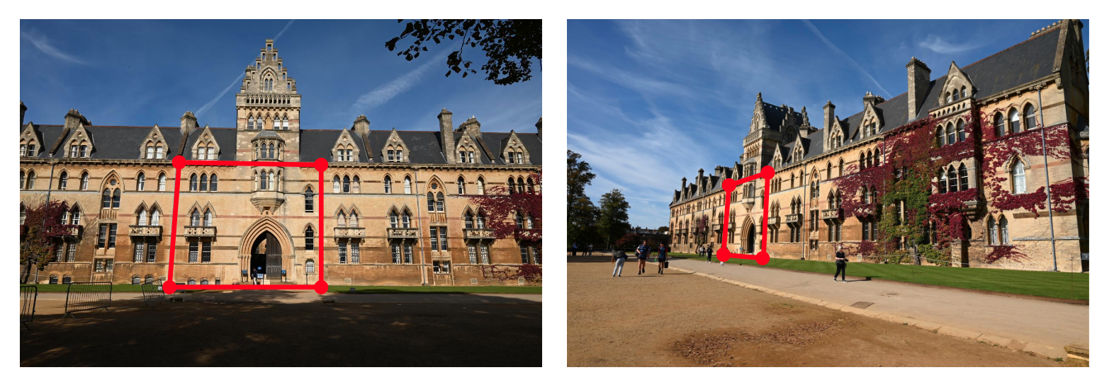
How many point-to-point correspondences are required to determine a homography?
$4$, as long as no $3$ points lie on the same line.
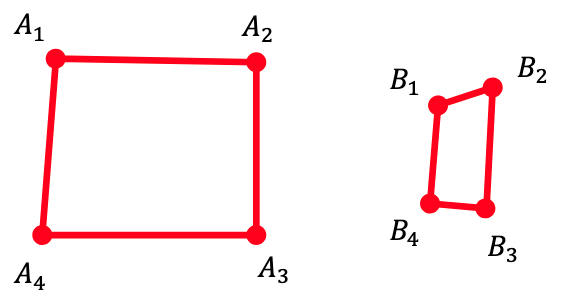
Suppose you have $4$ point-to-point correspondences $A _ 1, A _ 2, A _ 3, A _ 4$ and $B _ 1, B _ 2, B _ 3, B _ 4$.
Supposing that the entries of the homography matrix are
\[\begin{pmatrix}
h _ {11} & h _ {12} & h _ {13} \\
h _ {21} & h _ {22} & h _ {23} \\
h _ {31} & h _ {32} & h _ {33}
\end{pmatrix}\]
how could you solve for $H$?
Writing the correspondences down and then collecting them into a linear system, we have
\[\begin{pmatrix} - A _ {x,1} & - A _ {y,1} & -1 & 0 & 0 & 0 & B _ {x,1}A _ {x,1} & B _ {x,1}A _ {y,1} & B _ {x,1} \\ 0 & 0 & 0 & - A _ {x,1} & - A _ {y,1} & -1 & B _ {y,1}A _ {x,1} & B _ {y,1}A _ {y,1} & B _ {y,1} \\ - A _ {x,2} & - A _ {y,2} & -1 & 0 & 0 & 0 & B _ {x,2}A _ {x,2} & B _ {x,2}A _ {y,2} & B _ {x,2} \\ 0 & 0 & 0 & - A _ {x,2} & - A _ {y,2} & -1 & B _ {y,2}A _ {x,2} & B _ {y,2}A _ {y,2} & B _ {y,2} \\ \vdots & \vdots & \vdots & \vdots & \vdots & \vdots & \vdots & \vdots & \vdots \\ 0 & 0 & 0 & - A _ {x,4} & - A _ {y,4} & -1 & B _ {y,4}A _ {x,4} & B _ {y,4}A _ {y,4} & B _ {y,4} \end{pmatrix} \begin{pmatrix} h _ {11}\\ h _ {12}\\ h _ {13}\\ h _ {21}\\ h _ {22}\\ h _ {23}\\ h _ {31}\\ h _ {32}\\ h _ {33} \end{pmatrix} = 0\]Hence $H$ lies in the null space of this matrix, which can be found via the SVD.
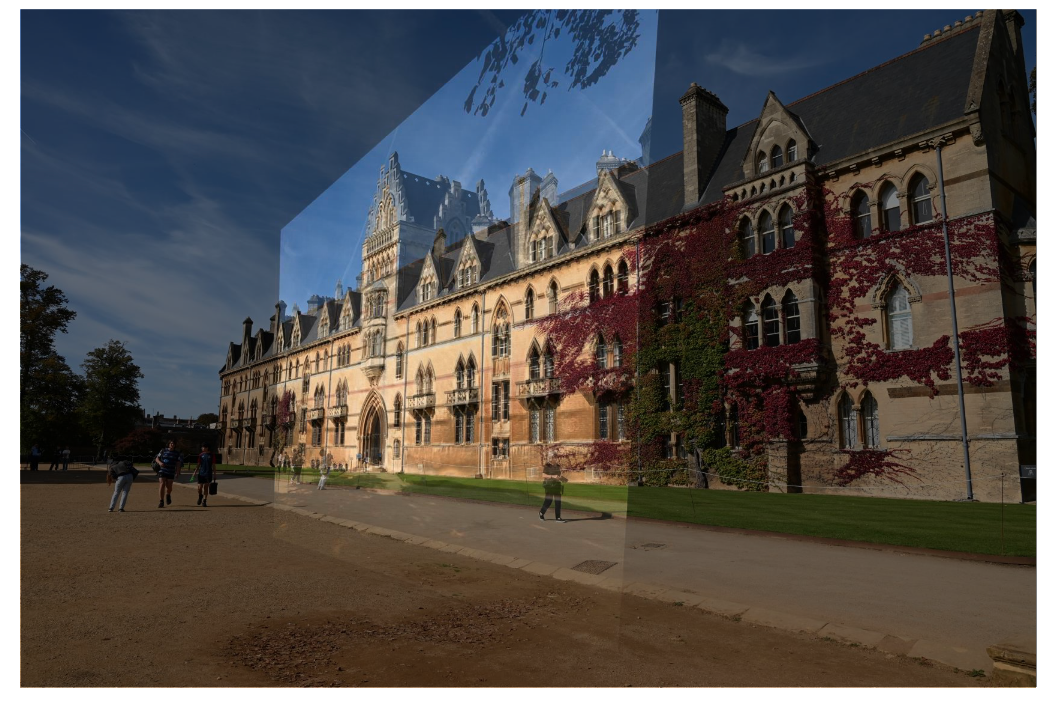
@Visualise how reversing the homography for the image on the right and overlaying the image on the left onto the image on the right would look.
How may a line $l$ be represented in homogenous coordinates?
Lines are defined via $ax + by + c = 0$, so taking $l= (a, b, c)^\top$ and $x = (x, y, 1)^\top$, we may write this as
\[l^\top x = 0\]@Define the cross product $a \times b$. How may it be written as a matrix multiplication?
Geometric meaning: $a \times b$ is perpendicular to both $a$ and $b$, with magnitude $ \vert a \vert \, \vert b \vert \,\sin\theta$, equal to the area of the parallelogram spanned by $a$ and $b$.
In homogeneous coordinates, @define $u \cong v$ for two vectors $u, v$.
$u, v$ are equal up to a non-zero scalar multiple.
Bite-sized
In homogeneous coordinates, a point with last coordinate $z = 0$ — for example $(x, y, 0)^\top$ — represents a point at infinity in the direction $(x, y)$. These are the “ideal points” that compactify the affine plane into the projective plane.
A homography has 8 degrees of freedom (a $3 \times 3$ matrix has 9 entries but is only defined up to scale). An affine transformation has 6 degrees of freedom (top two rows of a $3 \times 3$ matrix with last row $(0, 0, 1)$).
@Justify why affine transformations preserve parallelism but a general homography does not.
An affine map has the form $A \pmb x + \pmb t$ for some linear $A$ and translation $\pmb t$. Linear maps preserve linear combinations, and a translation acts uniformly on all points, so two parallel lines $\ell _ 1, \ell _ 2$ are sent to two lines that remain parallel.
A homography includes a perspective component (the bottom row of $H$ is not $(0, 0, 1)$). This causes points at infinity to map to finite points: the vanishing point. Concretely, two lines parallel in the source plane meet at the same point at infinity, but the homography sends that point to a finite vanishing point in the target — so the lines now intersect there. Hence parallelism is not preserved.
What is preserved by a general homography: collinearity, incidence, and the cross-ratio of four collinear points.
@Justify why a backward warp is generally preferred over a forward warp when applying a geometric transformation to an image.
- Forward warp $T(x, y) = (x', y')$: iterate over each source pixel and write it into the target at $(x', y')$. Two problems:
- Holes: many target pixels are never written (since $T$ may not map any integer source to them).
- Pile-ups: several source pixels can map to the same target — need to handle collisions.
- Backward warp $T^{-1}(x', y') = (x, y)$: iterate over each target pixel and look up its colour from the source. Every target pixel is written exactly once, no holes, no collisions. If the source coordinates are non-integer, interpolate (bilinear, bicubic, etc.).
The backward formulation is just an inverse-and-iterate, and it removes both of the forward-warp pathologies in a single move.
A homogeneous linear system $A \pmb p = \pmb 0$ subject to $\ \vert \pmb p\ \vert = 1$ is solved by taking $\pmb p$ to be the right singular vector of $A$ corresponding to its smallest singular value — equivalently the eigenvector of $A^\top A$ with the smallest eigenvalue. This is the SVD trick used to solve for the homography matrix, the fundamental matrix, and the camera projection matrix.
@Describe how composition of affine transformations works in homogeneous coordinates and why ordering matters.
In homogeneous coordinates, each affine transformation is a $3 \times 3$ matrix with bottom row $(0, 0, 1)$. The set of such matrices is closed under matrix multiplication — so composing two affine maps gives another affine map, and we just multiply their matrices.
Ordering: matrix multiplication is non-commutative. For a point $\pmb x$ expressed as a column vector, transformations are applied right-to-left: $R T \pmb x$ means “first translate by $T$, then rotate by $R$”. The example from the lecture:
\[R T = \begin{pmatrix} \cos\theta & -\sin\theta & \delta _ x\cos\theta - \delta _ y\sin\theta \\ \sin\theta & \cos\theta & \delta _ x\sin\theta + \delta _ y\cos\theta \\ 0 & 0 & 1 \end{pmatrix} \ne T R = \begin{pmatrix} \cos\theta & -\sin\theta & \delta _ x \\ \sin\theta & \cos\theta & \delta _ y \\ 0 & 0 & 1 \end{pmatrix}.\]So “translate then rotate” produces a different image to “rotate then translate”.
To convert from homogeneous coordinates $(x, y, w)^\top$ back to Euclidean 2D coordinates, divide by the last entry: $(x/w, y/w)$. This is the projection step in $\mathbb R^3 \to \mathbb R^2$ that gives perspective projection its $1/z$ depth dependence.
A line $\ell^\top \pmb x = 0$ in 2D homogeneous coordinates passes through two points $\pmb p _ 1, \pmb p _ 2$ iff $\ell$ is perpendicular to both — i.e. $\ell = <span class="cloze" tabindex="0">\pmb p _ 1 \times \pmb p _ 2</span>$. Dually, the intersection of two lines $\ell _ 1, \ell _ 2$ is the point $\pmb p = \ell _ 1 \times \ell _ 2$. This point-line duality via cross-product is the workhorse identity for projective geometry computations.