Numerical Analysis HT24, QR decomposition

\[A = QR\]

where $Q$ is orthogonal and $R$ is upper-triangular.

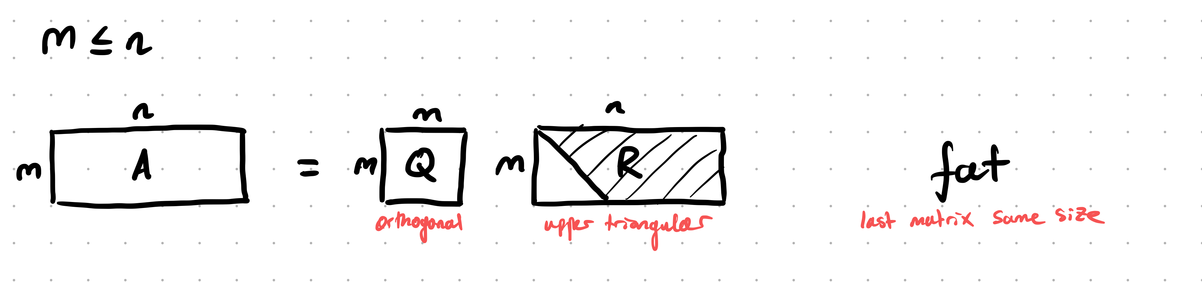
“Fat QR”: When $m \le n$, $A = QR$, $Q \in \mathbb R^{m \times m}$ and $R \in \mathbb R^{m \times n}$:

---

When $m \ge n$,

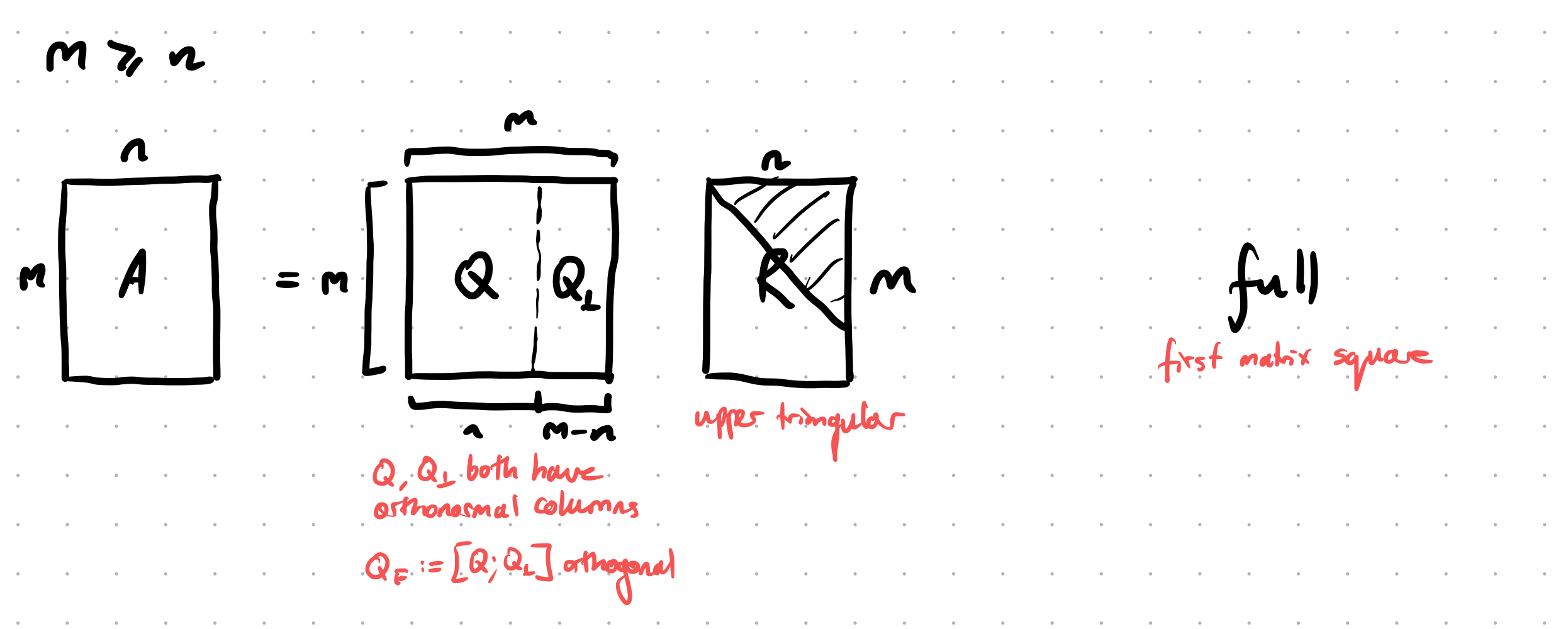
“Full QR”: $A = QR$, $Q \in \mathbb R^{m \times m}$ and $R \in \mathbb R^{m \times n}$, $Q$ is made to be square (and hence $Q$ is an orthogonal matrix):

---

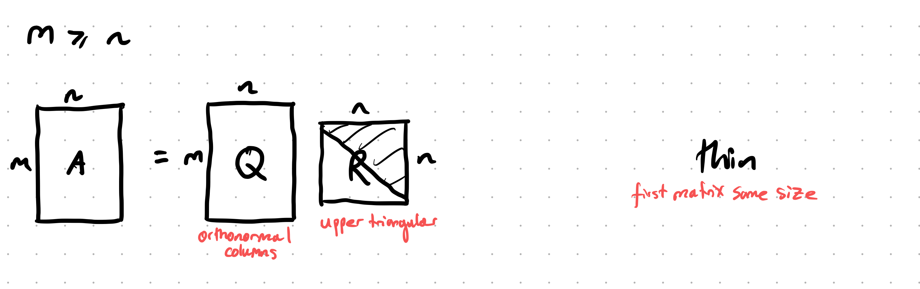
“Thin QR”: $A = QR$, $Q \in \mathbb R^{m \times n}$, $R \in \mathbb R^{n \times n}$, $Q$ is made to be the same size as the original matrix (and hence $Q$ has orthogonal columns, but isn’t an orthogonal matrix):

For the full QR, we have a factorisation

\[A = QR = \begin{bmatrix}Q _ 1 & Q _ 2\end{bmatrix} \begin{bmatrix}R \\\\ 0\end{bmatrix}\]

where $Q$ is an $m \times m$ matrix, and $R$ is a $m \times n$ matrix (i.e. $Q$ is made to be square, so it’s orthogonal).

In a thin QR, we have

\[A = Q'R'\]

where $Q’$ is the same size as $A$, namely $m \times n$, and $R’$ is $n \times n$.

They are related by the fact that

\[A = Q _ 1 R\]

is the thin QR factorisation.

$Q _ \perp$ is an “orthogonal extension” to $Q$, so all of its columns are orthogonal to the columns of $Q$.

Because orthogonal matrices are square matrices satisfying the property $Q^\top Q = I$, but $Q$ here is an $m \times n$ matrix with orthonormal columns.

\[Q^\top Q = I\]

but

\[QQ^\top \ne I\]

in general.

Yes. (Though this is not true if $Q$ is not square).

Suppose $A = Q _ 1 R _ 1$ and $A = Q _ 2 R _ 2$. Then

\[Q _ 2^{-1}Q _ 1 = R _ 2 R _ 1^{-1}\]

Since $R _ 2^{-1}$ is also upper triangular, $R _ 2^{-1} R _ 1$ is upper triangular. But $Q _ 2^{-1} Q _ 1$ is also orthogonal, so both of these matrices must be upper-triangular and orthogonal. But there is only one upper-triangular and orthogonal matrix, the identity ($\star$), so we are done.

($\star$: This is not immediate and needs proof).

We can turn the first column of a matrix into a vector like

\[\begin{pmatrix} \alpha \\ 0 \\ \vdots \\ 0 \end{pmatrix}\]

Continuing by induction and using block matrices like

\[\begin{pmatrix} 1 & 0 \\ 0 & H(w) \end{pmatrix}\]

we can annihilate all the sub-diagonal entries.

The modified Gram-Schmidt algorithm orthonormalises the columns of $A$, producing $A = QR$ with $Q$ orthonormal and $R$ upper triangular, computing the entries of $R$ as a by-product. “Modified” means each newly normalised $q _ i$ is subtracted from all the remaining columns immediately, rather than orthogonalising each column against all predecessors only at the end.

Algorithm: initialise $V = A = [v _ 1 \mid \cdots \mid v _ n]$ (the $v _ j$ are updated in place; $q _ i$ are the columns of $Q$).

• For $i = 1$ to $n$:
  • $r _ {i,i} = |v _ i| _ 2$ ($i$th diagonal entry of $R$; the length of the current $i$th column).
  • $q _ i = v _ i / r _ {i,i}$ (the $i$th orthonormal basis vector).
  • For $j = i+1$ to $n$:
    • $r _ {i,j} = q _ i^\ast v _ j$ (component of the remaining column $v _ j$ along $q _ i$; the $(i,j)$ entry of $R$).
    • $v _ j \leftarrow v _ j - r _ {i,j} q _ i$ (subtract that component now, so later columns are already orthogonal to $q _ i$).

Outputs:

• $Q = [q _ 1 \mid \cdots \mid q _ n] \in \mathbb R^{m \times n}$, orthonormal columns ($Q^\ast Q = I _ n$), with $\text{span}(Q) = \text{span}(A)$.
• $R \in \mathbb R^{n \times n}$ upper triangular, assembled from the computed scalars: $R _ {i,i} = r _ {i,i}$, $R _ {i,j} = r _ {i,j}$ for $i < j$, and $R_{i,j} = 0$ for $i > j$.

These satisfy $A = QR$, equivalently $R = Q^\ast A$.

Right-multiplication view: step $i$ is exactly right-multiplication by an upper-triangular $R _ i$, where $R _ i$ is the identity with its $i$th row replaced by $R _ i(i,j) = 0$ for $j < i$, $R_i(i,i) = 1/r_{i,i}$, and $R_i(i,j) = -r_{i,j}/r_{i,i}$ for $j > i$. The whole algorithm is then

\[Q = A\, R _ 1 R _ 2 \cdots R _ n,\]

so $R^{-1} = R _ 1 \cdots R _ n$ is upper triangular (a product of upper-triangular matrices), confirming $R$ is upper triangular. This is why Gram-Schmidt is triangular orthogonalisation.

Cost: $\approx 2mn^2$ flops to leading order (compare Householder QR’s $2mn^2 - \tfrac{2}{3}n^3$).

Caveat: classical Gram-Schmidt is numerically unstable, and even modified Gram-Schmidt loses orthogonality of the computed $\hat Q$ for ill-conditioned $A$ (∆why-not-gram-schmidt-for-qr), so Householder QR is preferred in practice.

Shared core: both build an orthonormal basis by taking each new vector, orthogonalising it against the previous basis vectors with modified Gram-Schmidt, normalising, and storing the orthogonalisation coefficients in a structured matrix.

Input vectors:

• Gram-Schmidt orthogonalises a fixed, given set of columns $a _ 1, \ldots, a _ n$ (all available up front).
• Arnoldi orthogonalises Krylov vectors generated on the fly: the next raw vector is $A q _ k$, which depends on the previous orthonormal vector, so the basis is built one matrix-vector product at a time.

Resulting structured factor:

• Gram-Schmidt produces an upper-triangular $R$ with $A = QR$ (equivalently $R = Q^\ast A$).
• Arnoldi produces an upper-Hessenberg $H _ k = Q _ k^\ast A Q _ k$ with $A Q _ k = Q _ {k+1} \tilde H _ k$. The one extra subdiagonal appears because $A q _ j$ has a component along the new direction $q _ {j+1}$.

Subspace:

• Gram-Schmidt: $\text{span}(Q) = \text{span}(A)$, the column space of the given matrix.
• Arnoldi: $\text{span}(Q _ k) = \mathcal K _ k(A, b)$, the Krylov subspace.

Cost: Gram-Schmidt $\approx 2mn^2$ for a dense $m \times n$ matrix; Arnoldi $O(nk^2)$ over $k$ steps plus $k$ matrix-vector products.

Stability: classical Gram-Schmidt loses orthogonality ($|\hat Q^\ast \hat Q - I| \le \epsilon \kappa _ 2(A)^2$), modified Gram-Schmidt is better ($\le \epsilon \kappa _ 2(A)$); Arnoldi uses the same modified-Gram-Schmidt core and inherits the same orthogonality loss, which is why reorthogonalisation is needed in Lanczos/Arnoldi.

In one phrase: Arnoldi is Gram-Schmidt applied to the Krylov sequence generated by $A$, producing a Hessenberg factor instead of a triangular one because the input vectors are produced by $A$ itself rather than given in advance.

Classical Gram-Schmidt loses orthogonality in floating-point: $|\hat Q^\top \hat Q - I| _ 2 \le \epsilon \kappa _ 2(A)^2$, so for ill-conditioned $A$ the computed $\hat Q$ can be far from orthogonal. Householder QR is unconditionally backward stable: $|\hat Q^\top \hat Q - I| _ 2 = O(\epsilon)$, regardless of $\kappa _ 2(A)$. The cost is essentially the same.